In this post, I’ll be reviewing a surface gradient bump mapping framework (jstor) proposed in 2020 by Dr. Mikkelsen (well-known also for creating the Mikktspace standard).

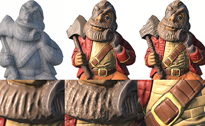
The objective of the framework is to provide a unified prescription for how to apply bump map influences from a variety of sources in a way that is consistent and comprehensible. In the example image taken from the paper below, the result on the right is the result of applying a tiled detail normal map on top of an unwrapped normal. Furthermore, the paper develops some math needed to blend a normal map influence without a dedicated vertex-frequency tangent space (as is the case for the secondary UV channel here).

While the paper and supporting work by the author is excellent (and recommended reading), I opted to write this post as a way to solidify my own understanding while hopefully offering some personal insight. Think of this post as a “retelling” of the original story, which will be necessarily lossy in some areas, but augmented with personal insights in others. Code snippets here are meant to be “illustrative” of the ideas, meaning they may be sloppy with respect to matters of precision or other aspects, so bear that in mind before adopting anything here in production. With that, we’ll start with an overview of bump mapping, jump straight to the “surface gradient idea”, and then discuss implementation and applications.

A brief note on notation

If you do opt to read the original paper (and you should), the author adopts several conventions that are worth bearing in mind:

• The author uses an overhead arrow $\vec{v}$ to denote a vector.
• A specific scalar component of a vector quantity looks like $\vec{v}_x$.
• Partial derivatives are often represented with subscripts (e.g. $\sigma_x$)
• A scalar-vector product looks like $s\cdot\vec{v}$ for some scalar field element \(s\) and vector $\vec{v}$.
• The dot-product between two vectors looks like $\vec{v}_1 \bullet \vec{v}_2$ (with a bigger centered dot symbol, typically reserved for bulleted lists).

In this post, I adopt the following notation instead.

• Vector quantities are shown in bold, so $\BF{n}$ is a vector.
• Lowercase symbols are either scalars or scalar fields based on context (e.g. $w$ is a scalar).
• A scalar component of a vector quantity drops the boldface (i.e. \(n_x\) is the x-component of $\BF{n}$).
• A partial derivative uses the partial symbol to distinguish derivatives from components (i.e. $\partial_x \sigma$ instead of $\sigma_x$).
• A vector scaled by a scalar looks like so: $w\BF{n}$
• A normalized unit vector has a hat: $\hat{\BF{n}} = \textrm{normalize}\left(\BF n\right)$
• A dot product between two vectors looks like so: $\BF{v}_1 \cdot \BF{v}_2$

At least for my personal tastes, I find that with the conventions as above, less time is spent deciphering the “type” of a given object. In addition, there is less confusion about whether a subscript is used to denote a vector component vs a derivative taken with respect to a variable. In agreement with the author and other differential geometry texts, I represent charts with lowercase Greek letters, and manifold surfaces with uppercase Roman letters (e.g. \(\phi\) could be a chart on the manifold \(M\)).

Bump mapping overview

Let’s remind ourselves what we’re trying to do in the first place. Artists would love to ship highly detailed 3D content, and a detailed appearance is composed of a variety of signals including:

• Albedo
• Microscopic roughness/metalness
• Geometry
• etc.

Geometric detail is often provided with variety of data sources, including but not limited to:

• Triangular meshes
• Heightfields
• Normal maps
• Signed distance fields
• etc.

Any of the above mechanism may be used (often in combination) to produce the position and orientation of the target surface for each pixel visible to the viewer. A reasonable question might be, “why are multiple sources of geometric information needed?” In practice, with 3D data, we quickly run into memory and processing constraints, and decoupling geometric data into different sources respresenting detail at different frequencies is a powerful tool to both compress the data, and improve renderer performance.

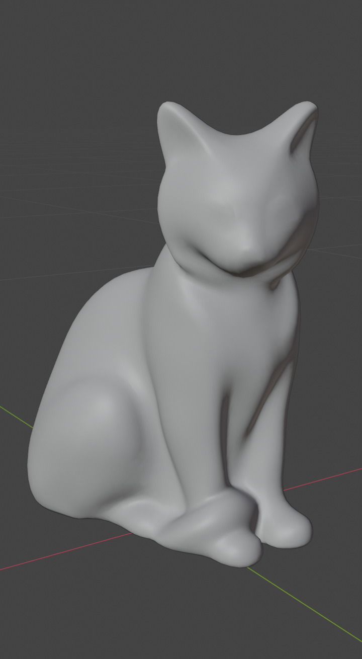
Above, we have a classic application of normal mapping. On the left, the mesh is visualized without any bump mapping applied. In the middle, a normal map is used to simulate a higher poly surface by perturbing the mesh normal based on a per-pixel normal map sample. The right-most image shows the rendered result, including other PBR channels. By decoupling some geometric detail into a normal map, we can represent a higher fidelity representation at pixel-frequency, as opposed to vertex- frequency.

Object-space normals

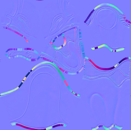
The normal map used above is unwrapped to the entire object as seen below. A specific set of faces is highlighted to demonstrate the correspondence between faces and the normal map.

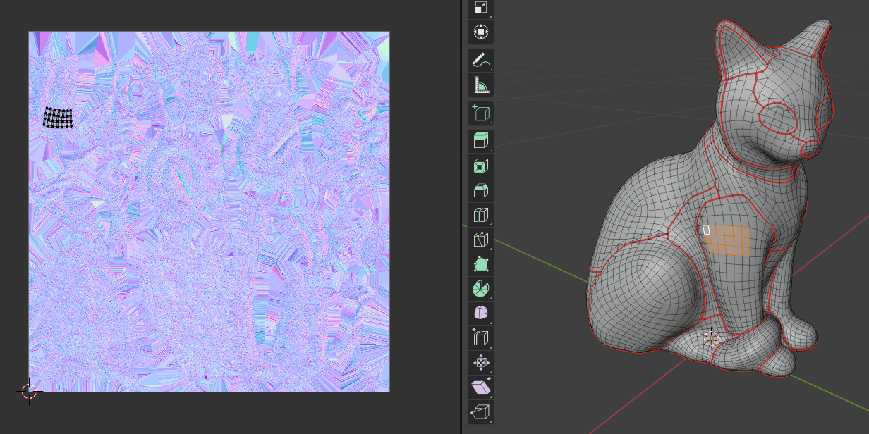
In this case, the normal map can be sampled and used directly as the surface normal in object space.

Tangent-space normals

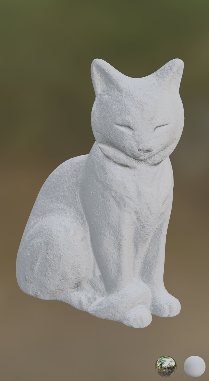
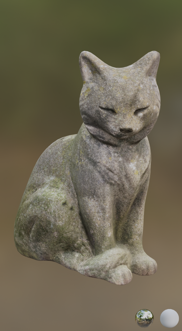
Things get significantly more complicated when we apply a normal map from a different surface. This is often the case when applying a tiling material as seen below:

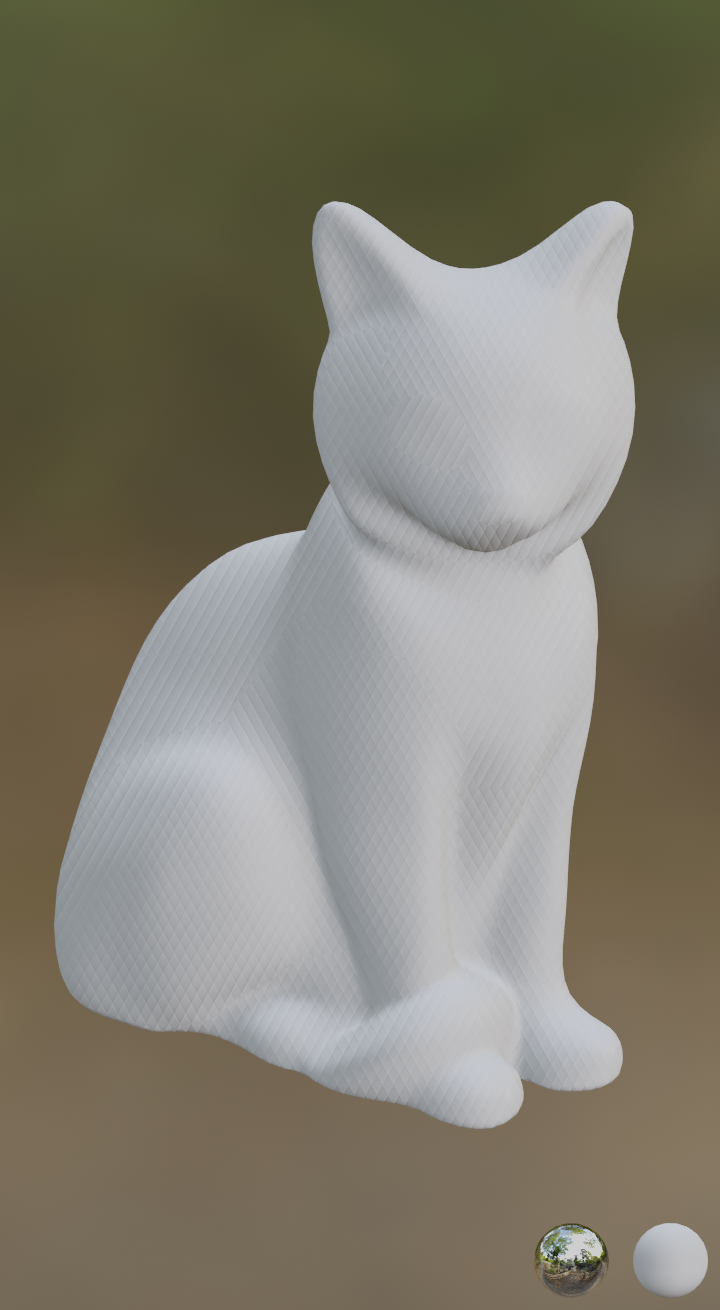
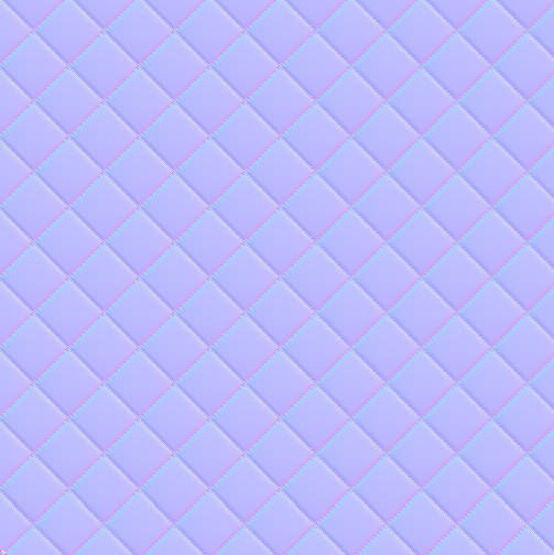
The cloth weave normal map tiled across the cat was baked from a different surface, and the orientation must be aligned to the surface of the cat before the sampled normals are applied.

Other common cases where tangent-space normals are needed are cases where the geometry is procedurally transformed at runtime in a non-rigid fashion, as is the case with skeletal mesh skinning or vertex morphing (also referred to as “blend shapes”). For example, the walking manniquin rendered below has a baked normal map (pictured right),

NOTE: The textures used for this mesh are technically incorrect and created for a different mesh altogether, but I didn’t notice while writing this post because I didn’t know what it was “supposed” to look like. Apologies to the artist!

As with object-space normal maps, in this example, the normal is sampled at each pixel. The difference is the normal sampled in this way cannot be used directly, and must be first transformed into the tangent space of the surface containing the pixel. This transformation may be encoded at vertex frequency (commonly referred to as vertex tangents), or as yet another image map (referred to as a tangent map). Failure to apply this transformation will result in something less than ideal.

Oops! Normals must be transformed into a consistent coordinate space!

Combining multiple bump influences

We already saw a tiling normal map in the cloth weave example above. In games, it’s common for several bump influences to be combined per-pixel. For example, you might do this to splat multiple material layers together when rendering terrain, composite deposits/decals on top of surfaces, or something else entirely.

Given multiple normals sampled or procedurally generated, the wrong way to produce the final per-pixel normal is to do a weighted average like:

The quantity $\hat\BF{n}^\prime$ is the symbol I use to refer to the “resolved normal” after all bump influences are accounted for. The linear blend here is likely the first thing someone would try, but doesn’t quite work the way an artist would anticipate. As a simple counterexample, consider the case when one of the local influences is completely “flat”. In tangent space, normals from such an influence are entirely vertical (blue). When blending this flat influence with some weight, we would expect the final result to be flattened in proportion to the weight. Instead however, the linear blend operation above would cause the overall result to be flattened (shifted blue), probably more than would be expected.

What we want instead, is a blend operation such that inputs that are locally flat produce no contributions to the final result. Ideally, we also want the blend to be a linear operation as well. We’ll get into this more later when we examine the mechanics of the surface gradient approach. For a nice summary of previous approaches that have been used, feel free to check out this nice post from Stephen Hill.

More exotic applications

Of course, the examples above are just a small slice of the pie when it comes to how many ways we can sample normals and apply them. Aside from vertex or image-based tangent space encodings, there are times we may need to procedurally derive a tangent space, for example, when performing parallax occlusion mapping. In addition, there are volumetric techniques and cases where a surface parameterization is unavailable. Having a theoretical framework lets us adapt the technique to a variety of use-cases, and intermix techniques with consistent and predictable results.

Such a framework would need to easily adapt to existing techniques shown above, handle new cases, and impose little-to-no runtime performance penalties. At least… that’s the hope! So with the motivational bits and general overview out of the way, let’s dive into the surface gradient framework itself and see how it works.

The surface gradient framework

Previously, all sampling and blending operations were concerned with normals, which makes some sense to a degree. The normal vector at all points on a surface characterize the surface well, and the normal is ultimately what we need to light the surface (using quantities like $\hat\BF{n} \cdot \hat\BF{l}$ and $\hat\BF{n}\cdot \hat\BF{v}$). However, normals are an unwieldy object to work with mathematically. They are finnicky, requiring renormalization after computations are transformed, blend linearly but not in a way that produces a perceptually linear effect, and transform covariantly with the coordinate space. A far more convenient quantity to work with is the height of the perturbed surface at each point on the surface.

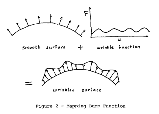
The idea of the perturbed surface can be seen above from Blinn’s original paper on the subject (pdf link). Traditionally, the normal vector of the perturbed surface seen above is stored and manipulated, but we’re going to work with the idea of the height of the perturbed surface instead. As we’ll see, we don’t need the height directly per se, but we can recover the gradient of the perturbed height based on existing quantities we’ve already seen.

With that in mind, let’s formalize what this height means a bit. We start with an unperturbed surface $S$ and one or more additional surfaces $S_1$, $S_2$, $\dots, S_i$ that we’d like to use to perturb the original surface. Assume for now that each surface possesses a surface parameterization (i.e. UV mapping) with a corresponding subscript, so that would be $\sigma$, $\sigma_1$, and so forth. Using these parameterizations (and with appropriate invertibility), given a point on $S$, we can determine the corresponding point on each of the other surfaces. Projecting corresponding points of any $S_i$ onto $S$ (i.e. with a raycast) gives us a scalar height $h_i$. In order to speak meaningfully about the orientation of this height, we ideally want to be able to take partial derivatives of $h_i$. The author does this by imagining a local extension to $h$ which is defined in a neighborhood around each point (pictured below).

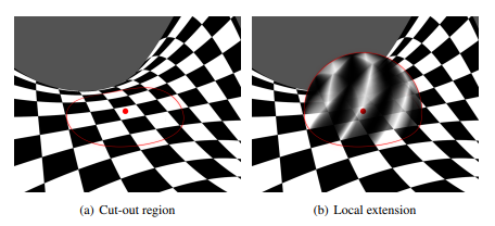
Without getting into any of the technical differential geometry (which would require us to define transitions between charts, stipulate smoothness, etc.), I’m just going to say that in all of $\mathbf{R}^3$, there is a scalar field $h_i$ that we can define which associates every point in space with a height associated with the influence of surface $S_i$. In practice, we really just need to imagine that such a hypothetical height field is available “wherever needed” to compute local derivatives on $S$.

Differentiability is critical, because derivatives give us “slopes” which are oriented orthogonally to normals. The author (and others, for example, Lovisach in Care and Feeding of Normal Vectors - pdf link) point out that the height gradients contain the same information that a normal does. If we consider $\BF\nabla_{S} h_i$ (the gradient of $h_i$ projected on $S$), this quantity is interpreted to be a vector in the direction with the greatest increase in $h_i$ on $S$. This vector is orthogonal to the normal vector we’d traditionally store in a normal map. Furthermore, we can recover the perturbed normal by subtracting this surface gradient from the unperturbed normal.

To see why this formula works conceptually, imagine perturbing a surface and consider how the normal vectors are biased in a direction based on steepness. At points where $\BF\nabla_{S} h_i$ are great, we expect large perturbations away from the slope, and at points where $\BF\nabla_{S} h_i$ are close to zero, we expect little to no perturbation of the normal at all.

With this idea, we can opt to work with height surface gradients as opposed to normals, and consolidate multiple influences in what the paper calls a normal resolve like so:

The summation on the right is the weighted sum of all perturbations due to each of the bump influences. This formulation is nice because we finally have a linear operator we can use to combine the influences. Compared to linearly scaling and blending normals, with this formulation, we are linearly scaling and blending the perturbations to the normal.

At this point, a somewhat obvious problem is that we need to somehow compute (or store) the surface gradients. As discussed previously though, the surface gradient contains the same information that the perturbed normal does, and it’s quite easy to recover one from the other. Following the paper more closely now, let’s walk through how we’d compute the surface gradients in various scenarios.

Surface gradient from tangent-space normal vector with a tangent basis

In a pixel shader, we will often have quantities T and B available which represent the partial derivatives of the position with respect to texture coordinates u and v. These quantities are typically interpolated from vertex attribute data, and emitted as part of the mesh baking process. Furthermore, suppose we have a sampled quantity tN from the normal map (tN being shorthand for tangent-space normal) as well as the surface normal N. Typically, we’d compute the perturbed normal pN with an expression like pN = normalize(tN.x * T + tN.y * B + tN.z * N), effectively transforming the sampled normal into the tangent coordinate space.

In the current form, we don’t yet see what quantity corresponds to the height surface gradient required by the framework. Fortunately, we can massage the equation with a little bit of sleight of hand into the perturbation form. Going from code back to math notation, with T as $\BF{t}$, B as $\BF{b}$, N as $\hat\BF{n}$, pN as $\hat\BF{n}^\prime$, and tN as $\hat\BF{m}$ (the perturbed normal for surface $M$), we can write:

Note that to go from the first to the second line, we take advantage of the fact that multiplying the argument of a $\textrm{normalize}$ operator with any non-zero scalar quantity does not change the result (up to a sign). By dividing all addends in the argument by $m_z$, the rest is relatively straightforward. When implementing this function, the author opts to constrain $m_z$ to be positive (or the orientation of the perturbed normal would flip also). In addition, the ratios $\frac{m_x}{m_z}$ and $\frac{m_y}{m_z}$ are constrained within the interval from -128 to 128.

To summarize this section, when combining bump influences, if one such influence is the tangent-space normal which we’d traditionally have unwrapped to an object, we can recover the surface gradient using the expression above. As the author points out, we don’t need an actual height field to derive the height surface gradient (referred to in the paper as a “conceptual prior”). This pattern of massaging an expression to recover the surface gradient form is a recurring theme in the paper, and useful to understand. From here, we’ll continue to other cases, but note that if you are using the mikkTSpace convention for baking vertex-frequency tangent spaces, a conditioning step on T, B, and N is necessary which we’ll discuss later.

Surface gradient from a tangent-space normal vector without an explicit tangent basis

In this use case, we have a surface parameterization, and a normal vector corresponding to a perturbed surface, but no known tangent basis. To use the result in the section above, we need to derive a tangent basis using available information. In a pixel or compute shader (with SM 6.6), we can take partial derivatives of the position with respect to the screenspace using the ddx and ddy intrinsics.

The goal is to recover expressions for $\BF{t}$ and $\BF{b}$ at point $\BF{p}$, which represent partial derivatives of the surface position with respect to the surface parameterization. Furthermore, these vectors are expected to lie in the tangent plane at $\BF{p}$. Assuming we have a normalized interpolated normal vector $\hat\BF{n}$, $\hat\BF{b}$ can be computed in terms of $\BF{t}$ and $\BF{n}$.

Here, the projection operator denoted $\textrm{proj}_S$ is the projection of the argument vector onto the surface $S$. Changing the variable with which we take a partial with respect to requires an application of the chain rule.

Here, $x$ and $y$ are the screenspace x and y coordinates respectively. Also, for now we’ll write $\BF t$ instead of $\hat\BF t$ and drop the normalization operation. Using the linearity of the projection operator lets us do some quick simplifications:

At this point, however, we still don’t have this in a form where ddx and ddy are immediately usable. You may be tempted to take the reciprocals of ddx(uv).x and ddy(uv).x to be the partials of $x$ and $y$ with respect to $u$, but this would be incorrect here (it’s true in the 1-dimensional case, or when the variables are independent). The “inverse” partials must be computed by computing the inverse of the Jacobian matrix.

In this case, the Jacobian matrix of our parameterization with respect to screenspace can be written as:

Note that I’ve switched to the shorthand form of the partial derivative for brevity. A fact from multivariable calculus (given by the Inverse Function Theorem) lets us write:

Substituting these quantities into our equation for $\BF t$:

A fact from before that we can use is that if a vector is going to be normalized anyways, we can carefully drop scalar multipliers but not sign changes prior to the normalization. This gives us our final expression for the normalized tangent vector:

Here, $\left|\BF J\right|$ is the Jacobian itself (aka, the determinant of the Jacobian matrix). In HLSL code, we could express this like so:

struct TangentFrame
{
  float3 t;
  float3 b;
  float3 n;
};

// Given:
// p - world-space pixel position
// n - (normalized) world-space surface normal
// uv - surface coordinates
TangentFrame compute_tbn(in float3 p, in float3 n, in float2 uv)
{
  float3 dpdx = ddx(p);
  float3 dpdy = ddy(p);

  // Project the position gradients onto the tangent plane
  float3 dpdx_s = dpdx - dot(dpdx, n) * n;
  float3 dpdy_s = dpdy - dot(dpdy, n) * n;

  // Compute the jacobian matrix to leverage the chain rule
  float2 duvdx = ddx(uv);
  float2 duvdy = ddy(uv);
  float jacobian_sign = sign(duvdx.x * duvdy.y - duvdx.y * duvdy.x);

  TangentFrame frame;
  frame.t = jacobian_sign * (duvdy.y * dpdx_s - duvdx.y * dpdy_s);

  // The sign intrinsic returns 0 if the argument is 0
  if (jacobian_sign != 0.0)
  {
    frame.t = normalize(frame.t);
  }

  // The second factor here ensures a consistent handedness between
  // the tangent frame and surface basis w.r.t. screenspace.
  frame.b = jacobian_sign *
    sign(dot(dpdy, cross(n, dpdx))) *
    cross(n, frame.t);

  frame.n = n;

  return frame;
}

Hopefully, you should be able to see the correspondance between the equation above and the implementation given here. Note that for precision purposes, it likely makes sense to operate in a coordinate space that shifts the world origin to the camera (but keeping the same orientation as the world’s coordinate space).

With the tangent frame produced here, the sampled normal can be converted into the surface gradient form as in the previous section.

To prove that this works, I constructed two materials using Unreal Engine sample content, both using the same color and normal map. In one version of the material, I sample the normal map and use the built-in mikkTSpace-based reconstruction. In the other version, I disable tangent-space normals and use the function above to compute the normal in world space. Below is a side-by-side of the two materials applied to a skinned mesh.

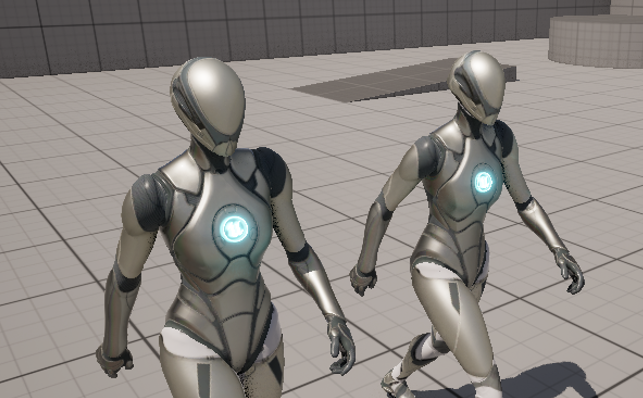
The mesh above on the left was rendered without using the baked vertex tangent. Unreal users should note that a DeriveTangentBasis material function is available, but this function doesn’t project the position gradients onto the tangent plane based on the interpolated normal. In addition, this material function omits the sign-corrections which may cause a reconstruction failure when using with double-sided or procedural geometry. 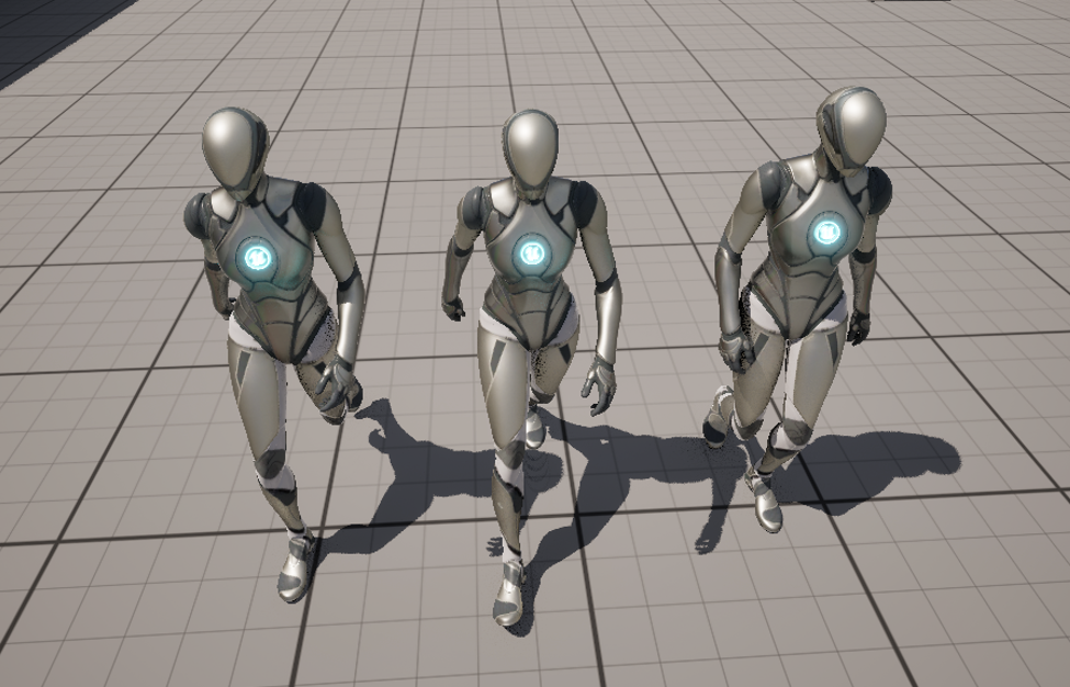For some types of geometry however, these omissions may be justified to save multiple instructions per-pixel. Below, a material based on the built-in DeriveTangentBasis is used on the skinned mesh on the far left.

Volumetric bump maps

An artist-defined volumetric bump map gives us a true 3D scalar field $h$ which defines a height displacement at each point. This implies that determining the per-pixel gradients are quite simple, and the only remaining step is to project the gradient onto the surface.

A note on mikkTSpace usage

In the formulas seen above, we always used a normalized surface normal vector $\hat\BF n$. However, the mikkTSpace encoded normal vectors are reconstructed assuming that the interpolated tangent, bitangent, and normal are not normalized.

// mikkTSpace reconstruction from mikktspace.com
vB = sign * cross(vN, vT);
vNout = normalize( vNt.x * vT + vNt.y * vB + vNt.z * vN );

This poses a problem for us because we can’t use the interpolated normal (vN here) as is. As a reminder for why this reconstruction is important, remember that the normal map baker has a choice about how to encode normals per-texel. Texels will generally lie “in between” vertices when a general surface parameterization is considered, and for each texel, we can encode the normal with respect to “some” tangent basis. By using the mikkTSpace tangent space averaging weighting rules per-vertex, and encoding the normal using the un-normalized interpolated tangent frames between vertices, we can encode a normal vector that is easily decoded using the code snippet above.

The method to recover “mikkTSpace compliance” during reconstruction but with a normalized normal vector is to use the length of vN to correct the lengths of vT and vB. Yet again, we use the trick that an unsigned scalar multiplier applied to the argument of a normalization operation does not change the result.

vB = sign * cross(vN, vT);

float inv_length_n = 1.0 / length(vN);

vT *= inv_length_n;
vB *= inv_length_n;
vN *= inv_length_n; // vN is now normalized

// Note that if we later reconstruct a sampled tangent-space normal like so:
vNout = normalize( vNt.x * vT + vNt.y * vB + vNt.z * vN );

// vNout matches the previous snippet because all terms in the normalize
// argument were scaled by the same unsigned quantity.

This “renormalization” should be performed before leveraging any interpolated quantities in the surface gradient derivations.

Summary and parting thoughts

I am a huge fan of this paper, and related papers that came before it. If you wanted a short list of insights and takeaways, I would try to remember the following:

• Instead of blending normals directly, think instead of blending perturbations to a normal.
• The actual bump influences should be a function of the implicit perturbed surface, but not the parameterization.
• Take advantage of normalization operations in your derivations to ditch unnecessary factors (in the same vein as Finish your derivations, please).
• Converting all bump influences into height surface gradients lets us blend influences in a consistent and artist-friendly way.

In this summary, I glossed over a number of details, opting instead to move slower through what I considered to be the “essential” parts. The paper itself covers far more use cases and applications, which I believe come naturally once the core ideas are understood. Some of these details include:

• How do we construct a tangent frame if ddx and ddy are unavailable?
• How do we account for scale-dependent tiling?
• How do we compute surface gradients given a height map?
• How do we compute surface gradients in the case of parallax occlusion mapping?
• How can we make additional perturbations to a post-resolved normal?

The last two items in particular, I encourage you to work through on your own, as it’s a nice test of your ability to reorient your thinking around “height gradients” as opposed to strictly normals. The paper is there for you to check your work, as well as helpful sample code here.

And with that, I’ll leave you with a few links I’ve found useful to digest this type of content over the years:

• Differential Geometry of Curves and Surfaces (Amazon, non-affiliate): My favorite book on differential geometry that I used during undergrad
• Discrete Differential Geometry: An Applied Introduction: An awesome discrete treatement of differential geometry from Keenan Crane
• Simulation of Wrinkled Surfaces (pdf): Blinn’s original treatment on bump mapping
• Care and Feeding of Normal Vectors (pdf): A GDC 2008 talk from Loviscach that also discusses the height-based formulation
• Simulation of Wrinkled Surfaces Revisited (pdf): Mikkelsen’s thesis which motivates mikkTSpace while also developing the prerequisite differential geometry background and covering additional topics
• Blending in Detail (blog): A blog post covering a variety of different methods for blending normal maps encountered in the wild
• Bump Mapping Unparameterized Surfaces on the GPU (pdf): Mikkelsen describing how to apply bump mapping if no parameterization is available
• Surface Gradient-Based Bump Mapping Framework (jstor): The paper of interest in this post (also by Mikkelsen)