Tangent Spaces and Diamond Encoding

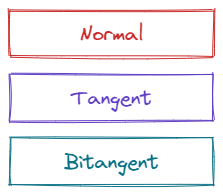
In this post, I wanted to touch briefly on tangent space encodings in mesh vertices and gbuffers. Intuitively, a full float3 normal, float3 tangent, and float3 bitangent (not a binormal, which is a different thing entirely), is not a very efficient representation. Here, I’ll present two ideas I haven’t seen discussed elsewhere (apologies if I missed it). If you’re already familiar with tangent space encodings, feel free to skip to the sections at the end.

Tangent Space Review

As a quick review, the ultimate goal of a tangent space is to enable bump-mapping of some sort. The basic idea is to perturb the normals of a surface “somehow,” thereby creating the illusion of more geometric detail than is actually present in the underlying geometry. These normal perturbations are typically stored in a “normal map” or “normal texture” and sampled at material evaluation time.

In order to ensure normal maps are reusable across different meshes, they are typically encoded in the surface coordinate space as opposed to object or world space (although world and object space encodings were used in early bump mapping developments). The tangent space itself is a concept from differential geometry - to visualize it, imagine associating set of coordinate axes with every point on the surface of a mesh. The coordinate axes should have two axes which lie in the unique plane tangent to its associated point (refer to these as the tangent $T$ and the bitangent $B$). The final coordinate axes should be orthogonal to that tangent plane (aka the normal).

We’d like to represent the artist-authored tangent space at each vertex in as compact a representation as is reasonable, without sacrificing too much precision, and without incurring too much ALU cost during decode. Smaller vertex footprints means less GPU memory traffic, more space for more triangles, and ultimately shipped content with higher fidelity.

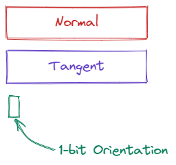
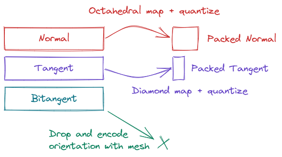
Assuming the normal vector is provided at each vertex, we still have a couple degrees of freedom. First, we haven’t stipulated that $T$ and $B$ be orthogonal, and further, we haven’t actually placed them on the tangent plane yet. By convention, we point $T$ in the direction where the first texture coordinate changes the most rapidly, and $B$ in the direction where the second texture coordinate changes the most rapidly. In practice, many renderers assume $T$, $B$, and $N$ form an orthonormal basis (henceforth abbreviated “TBN”), and not accounting for the skew typically doesn’t result in objectionable artifacts. This means we can immediately drop $B$ from our representation - except that we don’t know the handedness of the basis yet. Usually, a bit is reserved to indicate if the tangent basis is mirrored or not, but we will revisit this later.

As an aside, some content will require non-orthogonal and non-unit tangents and bitangents. These requirements can be met with a few adjustments which we’ll discuss later, but for now, assume that $T$, $B$, and $N$ are all mutually orthogonal and unit-length.

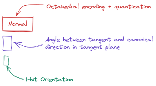
Currently, our encoding has gone from 9 floats, to 6 floats and a single bit for the orientation. The next thing to consider is encoding the normal.

The Effective Octahedral Encoding

Before continuing, if you haven’t checked out this excellent survey on encoding 3D unit vectors, I highly recommend giving it a skim. If that’s too much trouble, the main upshot is that octahedral encoding gives you the best bang for the buck out of the approaches suggested.

To see why, recall that a float3 vector essentially spans all of $\mathbf{R}^3$ with 12 bytes of memory. This is, of course, quite wasteful because a unit-length vector will never be in the interior or exterior of the unit sphere. Thus, we’d like to find a mapping that strictly encodes points on the unit sphere, and nothing else.

A naive way of doing this is using spherical coordinates, but you’ll quickly find that because of clustering, you end up losing precision away from the poles. This is covered extensively in the linked paper, but you can sort of see why the octahedral encoding works so well at a glance.

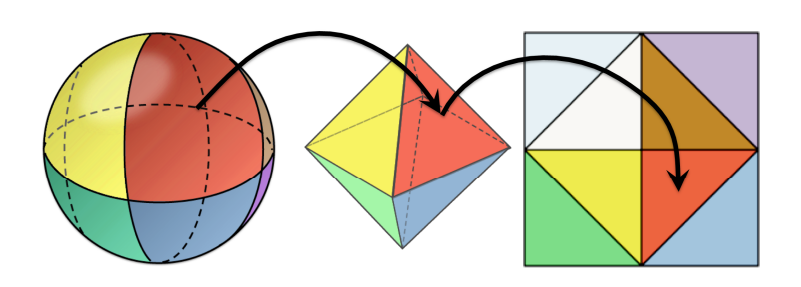
If you pay attention to the red face shown in the front, the first thing to consider is how much “warping” you’d need to turn the spherical wedge into the triangle (not much). The second thing to notice is how the unwrapping step preserves continuity across the boundaries of the different octants.

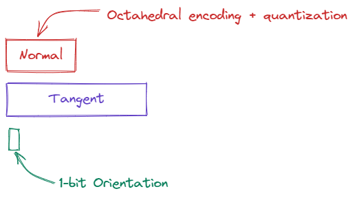
If we apply octahedral encoding to $N$, we can compress it from a float3 to a float2, and we can further quantize it from a float2 to an 8-bit or 16-bit snorm, depending on the level of accuracy needed.

Now, we’ve gone from 9 floats, to 3 floats, a 1-bit orientation, and two 16-bit snorms.

Encoding the Tangent with an Angle

To continue the encoding exercise, we now need to consider $T$. We know $T$ is orthogonal to $N$, so by the reasoning before, a full float3 representation is quite wasteful. We want an encoding that is restricted to the set of points orthogonal (and unit length) to the normal. A natural choice for this is to use an angle from a canonical direction.

This has been used to good effect in several titles (God of War and DOOM to name a few). The approach described in DOOM, for example, was presented in the Advances in RTR course at SIGGRAPH in 2020 here (PDF link).

To summarize the approach, first, we need to decide how to pick a canonical direction to encode our angle with respect to. DOOM uses the following choice:

Here, $T^\prime$ is what I’m calling the “canonical direction” in the tangent plane. It’s trivial to check that both cases are orthogonal to $N$. The conditions ensure that we pick reasonable directions that avoid any singularities as well. Determining the angle between $T$ and $T^\prime$ is then just an exercise in trigonometry by taking atan2 of the projection and rejection of $T$ onto and off $T^\prime$ (thanks Nathan Reed for the correction here from the original text). Note that we can choose the canonical direction in an infinite number of ways (albeit far fewer sensible ways), but I’m just reproducing the top approach for consistency.

edit As suggested by Marc Reynolds, there are a few other approaches linked to construct a canonical orthonormal basis, including this elegant solution from Pixar.

To reconstruct $T$ given $N$ and $\theta$, we need to determine $T^\prime$ using the same method as above, and then rotate $\theta$ radians about $N$ from $T^\prime$ using the Rodrigues rotation formula. As pointed out by the the DOOM presentation, the formula simplifies a bit since $T^\prime$ and $N$ are orthogonal. The reconstructed $T$ is computed as:

The angle itself can of course be quantized to a unorm (remember to scale by $2\pi$ later), so we’ve now compressed our tangent space quite a bit to 32-bit octahedral normal, 16-bit angle, and 1-bit orientation (of course, you can quantize more aggressively if your content allows).

“Diamond Encoding”

If there was a drawback to the angle-based approach given above, it’s that reconstructing $T$ requires invoking two transcendental functions. Other than that, it’s a great approach because unlike the spherical coordinate encoding, a planar angle is uniformly distributed throughout its range.

However, it occurred to me that we could simply apply the same trick used in octahedral encoding in a 2D sense. I’m calling it “diamond encoding” or “diamond mapping” for lack of a better term, but I will amend this article if I see it used elsewhere. The idea is basically to visualize a diamond embedded in the unit circle as below.

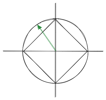
I’ve drawn a unit vector I’ll call $v$ to see how this works. If you imagine the intersection between $v$ and the diamond, you can then take the $x$ coordinate of that intersection to represent all the points in the upper quadrants. Of course, we also need to represent the lower quadrants also, so to do that, we simply squish the range $[-1, 1]$ to $[0.5, 1]$ for the upper two quadrants, and squish the bottom two quadrants into the lower half $[0, 0.5)$.

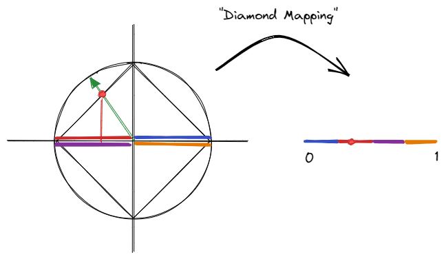
In the picture above, I tried to show how a point of the circle is projected onto the diamond, subsequently projected to the $x$-axis, and then remapped somewhere in the range $[0, 1]$. The color coding shows how each quadrant is mapped, and note that the mapping is continuous modulo $1$. To map the bottom quadrants, a minus-sign is needed to reverse the direction. This isn’t particularly novel, given that it’s just a 2D analogue of the octahedral mapping, but that means it’s fairly straightforward to understand and implement.

Decoding the diamond map is very similar to the angle-based encoding. As before, we find a canonical direction $T^\prime$ somewhere in the tangent plane. Next, we use $T^\prime \times N$ to construct another vector I’ll simply call $T^{\prime\prime}$. Together, $T^\prime$ and $T^{\prime\prime}$ span the tangent plane, and it is the coordinates of $T$ with respect to this basis of $T^\prime$ and $T^{\prime\prime}$ that we encode and decode. Once the projection is reversed so that we are again on the diamond, normalizing the vector once again takes us to the unit circle (as with the octahedral decoding).

If the explanation was too dry, here’s some sample code to demonstrate the idea (without quantization applied):

float encode_diamond(float2 p)
{
    // Project to the unit diamond, then to the x-axis.
    float x = p.x / (abs(p.x) + abs(p.y));

    // Contract the x coordinate by a factor of 4 to represent all 4 quadrants in
    // the unit range and remap
    float py_sign = sign(p.y);
    return -py_sign * 0.25f * x + 0.5f + py_sign * 0.25f;
}

float2 decode_diamond(float p)
{
    float2 v;

    // Remap p to the appropriate segment on the diamond
    float p_sign = sign(p - 0.5f);
    v.x = -p_sign * 4.f * p + 1.f + p_sign * 2.f;
    v.y = p_sign * (1.f - abs(v.x));

    // Normalization extends the point on the diamond back to the unit circle
    return normalize(v);
}

// Given a normal and tangent vector, encode the tangent as a single float that can be
// subsequently quantized.
float encode_tangent(float3 normal, float3 tangent)
{
    // First, find a canonical direction in the tangent plane
    float3 t1;
    if (abs(normal.y) > abs(normal.z))
    {
        // Pick a canonical direction orthogonal to n with z = 0
        t1 = float3(normal.y, -normal.x, 0.f);
    }
    else
    {
        // Pick a canonical direction orthogonal to n with y = 0
        t1 = float3(normal.z, 0.f, -normal.x);
    }
    t1 = normalize(t1);

    // Construct t2 such that t1 and t2 span the plane
    float3 t2 = cross(t1, normal);

    // Decompose the tangent into two coordinates in the canonical basis
    float2 packed_tangent = float2(dot(tangent, t1), dot(tangent, t2));

    // Apply our diamond encoding to our two coordinates
    return encode_diamond(packed_tangent);
}

float3 decode_tangent(float3 normal, float diamond_tangent)
{
    // As in the encode step, find our canonical tangent basis span(t1, t2)
    float3 t1;
    if (abs(normal.y) > abs(normal.z))
    {
        t1 = float3(normal.y, -normal.x, 0.f);
    }
    else
    {
        t1 = float3(normal.z, 0.f, -normal.x);
    }
    t1 = normalize(t1);

    float3 t2 = cross(t1, normal);

    // Recover the coordinates used with t1 and t2
    float2 packed_tangent = decode_diamond(diamond_tangent);

    return packed_tangent.x * t1 + packed_tangent.y * t2;
}

Overall, encoding and decoding is very fast, and while the distribution isn’t as good as the perfectly uniform angle distribution, this choice may be appropriate in some use cases (and the quality is quite good so far in my testing, although I don’t have rigorous results yet).

If you’re reading this post so far and are thinking, “but my tangents and bitangents aren’t unit-length and orthogonal,” you will need to augment your payload with the lengths of $T$ and $B$ (likely quantized also), and instead of dropping $B$ entirely, you could encode its angle or diamond map in the same way we encoded $T$ above. In that sense, all these techniques are fairly general.

What about the orientation bit?

So, at this point, you’ve encoded your normals with octahedral encoding, you’ve dropped your bitangent which you’ll reconstruct with the cross product later, and you’ve replaced your tangent with a single angle or diamond-mapped value as shown above. Presumably, you’ve also quantized all the above so you have a fairly compact representation of your tangent space payload now. That still leaves the orientation bit, needed to determine the direction of $B$.

One option of course, is to pick a value in the scheme used so far, give it one less bit of precision, and pack the orientation bit there. As of recently however, I’ve found a different option to be preferable, which is to simply split meshes based on tangent space orientation. With each mesh, we issue a draw with uniform data indicating whether the tangent space is right-handed or left-handed. Then, we simply read the sign bit from the uniform data instead of the packed vertex payload.

Previously, we would have preferred to keep the geometry together, since we’re now adding more draws (in the worst case, we double our draw count). However, I would contend that the above approach is better today for a few reasons:

1. Not much content is mirrored anymore, since artists aren’t as memory constrained
2. The extra draws aren’t relevant if you submit your draws as meshlets and GPU cull them anyways

In short, I recommend dropping the orientation bit altogether, given that times have changed in terms of how content is authored. As a compromise, it’s possible to store the orientation bit per-meshlet, or at some other frequency.

Summary

This was a quick overview of various common and less common schemes for encoding tangent space data with your vertices. There’s plenty of other bits I didn’t cover, like choosing how to quantize values based on mesh bounding boxes, or packing texture coordinates where possible by tracking the maximum and minimum values used on import. Other ideas to consider include more aggressive quantization possible when using meshlets by exploiting local surface similarity. That will all have to be for another day!