C++ Neural Network in a Weekend
Zero Dependencies 💪
Content mirrored from the Github repository
Introduction
Would you like to write a neural network from start to finish? Are you perhaps shaky on some of the fundamental concepts and derivations, such as categorical cross-entropy loss or backpropagation? Alternatively, would you like an introduction to machine learning without relying on “magical” frameworks that seem to perform AI miracles with only a few lines of code (and just as little intuition)? If so, this article was written for you.
Deep learning as a technology and discipline has been booming. Nearly every facet of deep learning is teeming with progress and healthy competition to achieve state of the art performance and efficiency. It’s no surprise that resources tend to emphasize the “latest and greatest” in feats such as object recognition, natural language parsing, “deep fakes”, and more. In contrast, fewer resources expand as much on the practical engineering aspects of deep learning. That is, how should a deep learning framework be structured? How do you go about rolling your own infrastructure instead of relying on Keras, Pytorch, Tensorflow, or any of the other dominant frameworks? Whether you wish to write your own for learning purposes, or if you need to deploy a neural network on a constrained (i.e. embedded) device, there is plenty to be gained from authoring a neural network from scratch.
The neural network outlined here is hosted on github and has enough abstractions to vaguely resemble a production network, without being overly engineered as to be indigestible in a sitting or two. The training and test data provided is the venerable MNIST dataset of handwritten digits. While more exotic (and original) datasets exist, MNIST is chosen here because its sheer ubiquity guarantees you can find corresponding literature to help drive further experimentation, or troubleshoot when things go wrong.
Background
This section serves as a moderately high-level description of the major mathematical underpinnings of neural networks and may be safely skipped by those who prefer to jump straight to the code.
Suppose we have a task we would like a machine learning model to complete (e.g. recognizing handwritten digits). At a high level, we need to perform the following tasks:
- First, we must conceptualize the task as a “function” such that the inputs and outputs of the task can be described in a concrete mathematical sense (amenable for programmability).
- Second, we need a way to quantify the degree to which our model is performing poorly against a known set of correct answers. This is typically denoted as the loss or objective function of the model.
- Third, we need an optimization strategy which will describe how to adjust the model after feedback is provided regarding the model’s performance as per the loss function described above.
- Fourth, we need a regularization strategy to address inadvertently tuning the model with a high degree of specificity to our training data, at the cost of generalized performance when handling inputs not yet encountered.
- Fifth, we need an architecture for our model, including how inputs are transformed into outputs and an enumaration of all the adjustable parameters the model supports.
- Finally, we need a robust implementation that executes the above within memory and execution budgets, accounting for floating-point stability, reproducibility, and a number of other engineering-related matters.
Deep learning is distinct from other machine learning models in that the architecture is heavily over-parameterized and based on simpler building blocks as opposed to bespoke components. The building blocks used are neurons, or particular arrangements of neurons, typically organized as layers. Over the course of training a deep learning model, it is expected that features of the inputs are learned and manifested as various parameter values in these neurons. This is in contrast to traditional machine learning, where features are not learned, but implemented directly.
Categorical Cross-Entropy Loss
More concretely, the task at hand is to train a model to recognize a 28 by 28 pixel handwritten greyscale digit. For simplicity, our model will interpret the data as a flattened 784-dimensional vector. Instead of describing the architecture of the model first, we’ll start with understanding what the model should output and how to assess the model’s performance. The output of our model will be a 10-dimensional vector, representing the probability distribution of the supplied input. That is, each element of the output vector indicates the model’s estimation of the probability that the digit’s value matches the corresponding element index. For example, if the model outputs:
\[M(\mathbf{I}) = \left[0, 0, 0.5, 0.5, 0, 0, 0, 0, 0, 0\right]\]for some input image $\mathbf{I}$, we interpret this to mean that the model believes there is an equal chance of the examined digit to be a 2 or a 3.
Next, we should consider how to quantify the model’s loss. Suppose, for example, that the image $\mathbf{I}$ actually corresponded to the digit “7” (our model made a horrible prediction!), how might we penalize the model? In this case, we know that the actual probability distribution is the following:
\[\left[0, 0, 0, 0, 0, 0, 0, 1, 0, 0\right]\]This is known as a “one-hot” encoded vector, but it may be helpful to think of it as a probability distribution given a set of events that are mutually exclusive (a digit cannot be both a “7” and a “3” for instance).
Fortunately, information theory provides us some guidance on defining an easy-to-compute loss function which quantifies the dissimilarities between two probability distributions. If the probability of of an event $E$ is given as $P(E)$, then the entropy of this event is given as $-\log P(E)$. The negation ensures that this is a positive quantity, and by inspection, the entropy increases as an event becomes less likely. Conversely, in the limit as $P(E)$ approaches $1$, the entropy shrinks to $0$. While several interpretations of entropy are possible, the pertinent interpretation here is that entropy is a measure of the information conveyed when a particular event occurs. That the “sun rose this morning” is a fairly mundane observation but being told “the sun exploded” is sure to pique your attention. Because we are reasonably certain that the sun rises each morning (with near 100% confidence), that “the sun rises” is an event that conveys little additional information when it occurs.
Let’s consider next entropy in the context of a probability distribution. Given a discrete random variable $X$ which can take on values $x_0, \dots, x_{n-1}$ with probabilities $p(x_0), \dots, p(x_{n-1})$, the entropy of the random variable $X$ is defined as:
\[H(X) = -\sum_{x \in X} p(x) \log p(x)\]For example, suppose $W$ is a binary random variable that represents today’s weather which can either be “sunny” or “rainy” (a binary random variable). The entropy $H(W)$ can be given as:
\[H(W) = -S\log S - (1 - S) \log (1 - S)\]where $S$ is the probability of a sunny day, and hence $1 - S$ is the probability of a rainy day. As a binary random variable, the summation over weighted entropies expands to only two terms. What does this quantity mean? If we were to describe it in words, each term of the sum in the entropy calculation corresponds to the information of a particular event, weighted by the probability of the event. Thus, the entropy of the distribution is literally the expected amount of information contained in an event for a given distribution. If we plot $-S\log S - (1 - S) \log(1 - S)$ as a function of $S$, we will see something like this:
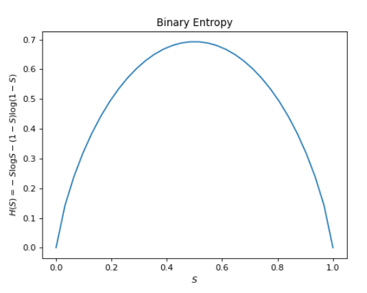
As a minor note, while $\log 0$ is an undefined quantity, information theorists accept that $\lim_{p\rightarrow 0} p\log p = 0$ by convention. Intuitively, the expected entropy should be unaffected by the set of impossible events.
As you might expect, when the distribution is 50-50, the uncertainty of a binary is maximal, and by extension the amount of information contained in each event is maximized too. Put another way, if you lived in an area where it was always sunny, you wouldn’t learn anything if someone told you it was sunny today. However, in a tropical region characterized by capricious weather, information conveyed about the weather is far more meaningful.
In the previous example, we weighted the event entropies according to the event’s probability distribution. What would happen if, instead, we used weights corresponding to a different probability distribution? This is known as the cross entropy:
\[H(p, q) = -\sum_{x \in X} p(x)\log q(x)\]To get some intuition about this, first, we note that if $p(x) = q(x), \forall x\in X$, the cross entropy trivially matches the self-entropy. Let’s go back to our binary entropy example and visualize what it looks like if we chose a completely incorrect distribution. Specifically, suppose we computed the cross entropy where if the probability of a sunny day is $S$, we weight the entropy with $1 - S$ instead of $S$ as in the self-entropy formula.
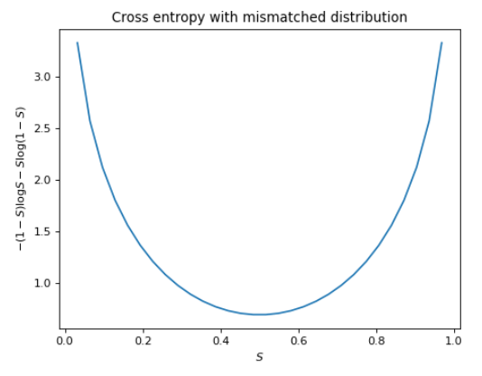
If you compare the values with the previous figure, you’ll see that the cross entropy diverges from the self-entropy everywhere except $0.5$, where $S = 1 - S$. The difference between the cross entropy $H(p, q)$ and entropy $H(p)$ provides then, a measure of error between the presumed distribution $q$ and the true distribution $p$. This difference is also known as the Kullback-Leibler divergence or KL divergence for short.
Given that the entropy of a given probability distribution $p$ is constant, then $H(p)$ must be constant as well. This is why in practice, we will generally seek to minimize the cross entropy between $p$ and a predicted distribution $q$, which by extension will minimize the Kullback-Leibler divergence as well.
Now, we have the tools to know if our model is succeeding or not! Given an estimation of a sample’s label as before:
\[M(\mathbf{I}) = \left[0, 0, 0.5, 0.5, 0, 0, 0, 0, 0, 0\right]\]we will treat our model’s output as a predicted probability distribution of the sample digit’s classification from 0 to 9. Then, we compute the cross entropy between this predction and the true distribution, which will be in the form of a one-hot vector. Supposing the actual digit is 3 in this particular case ($P(7) = 1$):
\[\sum_{x\in \{0,\dots, 9\}} -P(x) \log Q(x) = -P(3) \log(Q(3)) = \log(0.5) \approx 0.301\]Let’s make a few observations before continuing. First, for a one-hot vector, the entropy is 0 (can you see why?). Second, by pretending the correct digit above is $3$ and not, say, $7$, we conveniently avoided $\log 0$ showing up in the final expression. A common method to avoid this is to add a small $\epsilon$ to the log argument to avoid this singularity, but we’ll discuss this in more detail later.
Creating our Approximation Function with a Neural Network
Now that we know how to evaluate our model, we’ll need to decide how to go about making predictions in the form of a probability distribution. Our model will need to take as inputs, 28x28 images (which as mentioned before, will be flattened to 784x1 vectors for simplicity). Let’s enumerate the properties our model will need:
- Parameterization - our model will need parameters we can adjust to “fit” the model to the data
- Nonlinearity - it is assuredly not the case that the probability distribution can be modeled with a set of linear equations
- Differentiability - the gradient of our model’s output with respect to any given parameter indicates the impact of that parameter on the final result
There are an infinite number of functions that fit this criteria, but here, we’ll use a simple feedforward network with a single hidden layer.
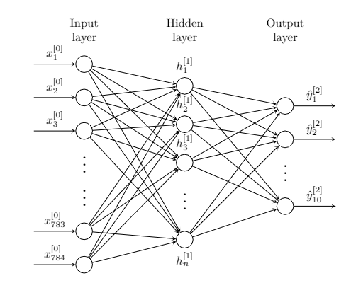
A few quick notes regarding notation: a superscript of the form $[i]$ is used to denote the $i$th layer. A subscript is used to denote a particular element within a layer or vector. The vector $\mathbf{x}$ is usually reserved for training samples, and the vector $\mathbf{y}$ is typically reserved for sample labels (i.e. the desired “answer” for a given sample). The vector $\hat{\mathbf{y}}$ is used to denote a model’s predicted labels for a given input.
On the far left, we have the input layer with $784$ nodes corresponding to each of the 28 by 28 pixels in an individual sample. Each $x_i^{(0)}$ is a floating point value between 0 and 1 inclusive. Because the data is encoded with 8 bits of precision, there are 256 possible values for each input. Each of the 784 input values fan out to each of the nodes in the hidden layer without modification.
In the center hidden layer, we have a variable number of nodes that each receive all 784 inputs, perform some processing, and fan out the result to the output nodes on the far right. That is, each node in the hidden layer transforms a $\mathbb{R}^{784}$ vector into a scalar output, so as a whole, the $n$ nodes collectively need to map $\mathbb{R}^\rightarrow \mathbb{R}^n$. The simplest way to do this is with an $n\times 784$ matrix (treating inputs as column vectors). Modeling the hidden layer this way, each of the $n$ nodes in the hidden layer is associated with a single row in our $\mathbb{R}^{n\times 784}$ matrix. Each entry of this matrix is referred to as a weight.
We still have two issues we need to address however. First, a matrix provides a linear mapping between two spaces, and linear maps take $0$ to $0$ (you can visualize such maps as planes through the origin). Thus, such fully-connected layers typically add a bias to each output node to turn the map into an affine map. This enables the model to respond zeroes in the input. Thus, the hidden layer as a whole has now both a weight matrix, and also a bias vector. A linear mapping with a constant bias is commonly referred to as an affine map.
The second issue is that our hidden layer’s now-affine mapping still scales linearly with the input, and one of our requirements for our approximation function was nonlinearity (a strict prerequisite for universality). Thus, we perform one final non-linear operation the result of the affine map. This is known as the activation function, and an infinite number of choices present itself here. In practice, the rectifier function, defined below, is a perennial choice.
\[f(x) = \max(0, x)\]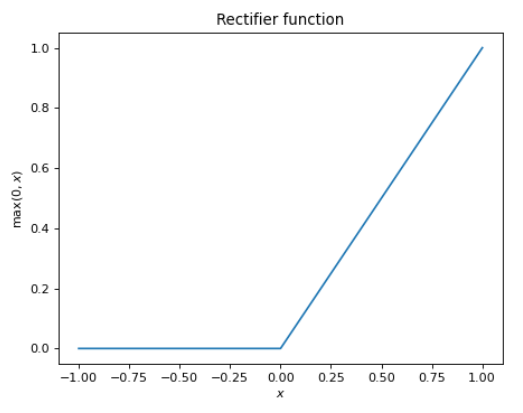
The rectifier is popular for having a number of desirable properties.
- Easy to compute
- Easy to differentiate (except at 0, which has not been found to be a problem in practice)
- Sparse activation, which aids in addressing model overfitting and “unlearning” useful weights
As our hidden layer units will use this rectifier just before emitting its final output to the next layer, our hidden units may be called rectified linear units or ReLUs for short.
Summarizing our hidden layer, the output of each unit in the layer can be written as:
\[a_i^{[1]} = \max(0, W_{i}^{[1]} \cdot \mathbf{x}^{[0]} + b_i^{[1]})\]It’s common to refer to the final activated output of a neural network layer as the vector $\mathbf{a}$, and the result of the internal affine map $\mathbf{z}$. Using this notation and considering the output of the hidden layer as a whole as a vector quantity, we can write:
\[\begin{aligned} \mathbf{z}^{[1]} &= \mathbf{W}^{[1]}\mathbf{x}^{[0]} + \mathbf{b}^{[1]} \\ \mathbf{a}^{[1]} &= \max(\mathbf{0}, \mathbf{z}^{[1]}) \\ \mathbf{a}^{[1]}, \mathbf{b}^{[1]} &\in \mathbb{R}^n \\ \mathbf{W}^{[1]} &\in \mathbb{R}^{n\times 784} \\ \mathbf{x}^{[0]} &\in \mathbb{R}^{784} \end{aligned}\]The last layer to consider is the output layer. As with the hidden layer, we need a dimensionality transform, in this case, taking vectors in $\mathbb{R}^n$ and mapping them to vectors in $\mathbb{R}^{10}$ (corresponding to the 10 possible digits in the target output). As before, we will use an affine map with the appropriately sized weight matrix and bias vector. Here, however, the rectifier isn’t suitable as an activation function because we want to emit a probability distribution. To be a valid probability distribution, each output of the hidden layer must be in the range $[0, 1]$, and the sum of all outputs must equal $1$. The most common activation function used to achieve this is the softmax function:
\[\mathrm{softmax}(\mathbf{z})_i = \frac{\exp(z_i)}{\sum_j \exp(z_j)}\]Given a vector input $z$, each component of the softmax output (as a vector quantity) is given as per the expression above. The exponential functions conveniently map negative numbers to positive numbers, and the denominator ensures that all outputs will be between 0 and 1, and sum to 1 as desired. There are other reasons why an exponential function is used here, stemming from our choice of a loss function (based on the underpinning notion of maximum-likelihood estimation), but we won’t get into that in too much detail here (consult the further reading section at the end to learn more). Suffice it to say that an additional benefit of the exponential function is its clean interaction with the logarithm used in our choice of loss function, especially when we will need to compute gradients in the next section.
Summarizing our neural network architecture, with two weight matrices and two bias vectors, we can construct two affine maps which map vectors in $\mathbb{R}^{784}$ to $\mathbb{R}^n$ to $\mathbb{R}^{10}$. Prior to forwarding the results of one affine map as the input of the next, we employ an activation function to add non-linearity to the model. First, we use a linear rectifier and second, we use a softmax function, ensuring that we end up with a nice discrete probability distribution with 10 possible events corresponding to the 10 digits.
Our network is small enough that we can actually write out the entire process as a single function using the notation we’ve built so far:
\[f(\mathbf{x}^{[0]}) = \mathbf{y}^{[2]} = \mathrm{softmax}\left(\mathbf{W}^{[2]}\left(\max\left(\mathbf{0}, \mathbf{W}^{[1]}\mathbf{x}^{[0]} + \mathbf{b}^{[1]}\right) \right) + \mathbf{b}^{[1]} \right)\]Optimizing our network
We now have a model given above which can turn our 784 dimensional inputs into a 10-element probability distribution, and we have a way to evaluate how accuracy of each prediction. Next, we need a reliable way to improve the model based on the feedback provided by our loss function. This is known as function optimization, and most methods of model optimization are based on the principle of gradient descent.
The idea is quite simple. Given a function with a set of parameters which we’ll denote $\bm{\theta}$, the partial derivative of that function with respect to a given parameter $\theta_i \in \bm{\theta}$ tells us the overall impact of $\theta_i$ on the final result. In our model, we have many parameters; each weight and bias constitutes an individually tunable parameter. Thus, our strategy should be, given a set of input samples, compute the loss our model produces for each sample. Then, compute the partial derivatives of that loss with respect to every parameter in our model. Finally, adjust each parameter in proportion to its impact on the final loss. Mathematically, this process is described below (note that the superscript $(i)$ is used to denote the $i$-th sample):
\[\begin{aligned} \mathrm{Total~Loss} &= \sum_i J(\mathbf{x}^{(i)}; \bm\theta) \\ \mathrm{Compute}~ &\sum_i \frac{\partial J(\mathbf{x}^{(i)})}{\partial \theta_j} ~\forall ~\theta_j \in \bm\theta \\ \mathrm{Adjust}~ & \theta_j \rightarrow \theta_j - \eta \sum_i \frac{\partial J(\mathbf{x}^{(i)})}{\partial \theta_j} ~\forall ~\theta_j \in\bm\theta\\ \end{aligned}\]Here, there is some flexibility in the choice of $\eta$, often referred to as the learning rate. A small $\eta$ promotes more conservative and accurate steps, but at the cost of our model being more costly to update. A large $\eta$ on the other hand results in larger updates to our model per training cycle, but may result in instability. Updating in the above fashion should adjust the model such that it will produce a smaller loss given the same inputs.
In practice, the size of the input set may be very large, rendering it intractable to evaluate the model on every single training sample in the sum above before adjusting parameters. Thus, a common strategy is to use stochastic gradient descent (abbrev. SGD) and perform loss-gradient-based adjustments after evaluating smaller batches of samples. Concretely, the MNIST handwritten digits database contains 60,000 training samples. If we were to train our model using gradient descent in the strictest sense, we would execute the following pseudocode:
model.init()

for i in num_training_cycles
    loss <- 0

    for n in 60000
        x <- MNIST.data[n]
        y <- model.predict(x)
        loss += loss(y, MNIST.labels[n])

    model.gradient_descent(loss)
In contrast, SGD pseudocode would look like:
model.init()

for i in num_batches
    loss <- 0
    for j in batch_size
        x <- MNIST.data[n]
        y <- model.predict(x)
        loss += loss(y, MNIST.labels[n])

    model.gradient_descent(loss)
SGD is very similar, but the batch size can be much smaller than the amount of training data available. This enables the model to get more frequent updates and waste fewer cycles especially at the start of training when the model is likely wildly inaccurate.
When it comes time to compute the gradients, we are fortunate to have made the prescient choice of constructing our model solely with elementary functions in a manner conducive to relatively painless differentiation. However, we still must exercise care as there is plenty of bookkeeping involved. We will evaluate loss-gradients with respect to individual parameters when we walkthrough the implementation later, but for now, let’s establish a few preliminary results.
Recall that our choice of loss function was the categorical cross entropy function, reproduced below:
\[J_{CE}(\mathbf{\hat{y}}, \mathbf{y}) = -\sum_{i} y_i \log{\hat{y}_i}\]The index $i$ is enumerated over the set of possible outcomes (i.e. the set of digits from 0 to 9). The quantities $y_i$ are the elements of the one-hot label corresponding to the correct outcome, and $\hat{\mathbf{y}}$ is the discrete probability distribution emitted by our model. We compute $\partial J_{CE}/\partial \hat{y}_i$ like so:
\[\frac{\partial J_{CE}}{\partial \hat{y}_i} = -\frac{y_i}{\hat{y}_i}\]Notice that for a one-hot vector, this partial derivative vanishes whenever $i$ corresponds to an incorrect outcome.
Working backwards in our model, we next provide the partial derivative of the softmax function:
\[\begin{aligned} \mathrm{softmax}(\mathbf{z})_i &= \frac{\exp{z_i}}{\sum_j \exp{z_j}} \\ \frac{\partial \left(\mathrm{softmax}(\mathbf{z})_i\right)}{\partial z_k} &= \begin{dcases} \frac{\left(\sum_j\exp{z_j}\right)\exp{z_i} - \exp{2z_i}}{\left(\sum_j\exp{z_j}\right)^2}& i = k \\ \frac{-\exp{z_i}\exp{z_k}}{\left(\sum_j\exp{z_j}\right)^2}& i \neq k \end{dcases} \\ &= \begin{cases} \mathrm{softmax}(\mathbf{z})_i\left(1 - \mathrm{softmax}(\mathbf{z})_i\right) & i = k \\ -\mathrm{softmax}(\mathbf{z})_i \mathrm{softmax}(\mathbf{z})_k & i \neq k \end{cases} \end{aligned}\]The last set of equations follow from factorizing and rearranging the expressions preceding it. It’s often confusing to newer practitioners that the partial derivative of softmax needs this unique treatment. The key observation is that softmax is a vector-function. It accepts a vector as an input and emits a vector as an output. It also “mixes” the input components, thereby imposing a functional dependence of every output component on every input component. The lone $\exp{z_i}$ in the numerator of the softmax equation creates an asymmetric dependence of the output component on the input components.
Finally, let’s consider the partial derivative of the linear rectifier.
\[\begin{aligned} \mathrm{ReLU}(z) &= \max(0, z) \\ \frac{\partial \mathrm{ReLU}(z)}{\partial z} &= \begin{cases} 0 & z < 0 \\ \mathrm{undefined} & z = 0 \\ z & z > 0 \end{cases} \end{aligned}\]While the partial derivative exactly at 0 is undefined, in practice, the derivative is simply assigned to 0. Why the non-differentiability at 0 isn’t an issue has been a subject of practical debate for a long time. Here is a simple line of thinking to justify the apparent issue. Consider a rectifier function that is nudged ever so slightly to the right such that the inflection point is $\epsilon / 2$, where $\epsilon$ is the smallest positive floating point number the machine can represent. In this case, the model will never produce a value that sits directly on this inflection point, and as far as the computer is concerned, we never encounter a point where this function is non-differentiable. We can even imagine an infinitesimal curve that smooths out the function at that inflection point if we want. Either way, experimentally, the linear rectifier remains one of the most effective activation functions for reasons mentioned, so we have no reason to discredit it over a technicality.
Now that we can compute partial derivatives of all the nonlinear functions in our neural network (and presumbly the linear functions as well), we are prepared to compute loss gradients with respect to any parameter in the network. Our tool of choice is the venerable chain rule of calculus:
\[\left.\frac{\partial f(g(x))}{\partial x}\right\rvert_x = \left.\frac{\partial f}{\partial g}\right\rvert_{g(x)} \left.\frac{\partial g}{\partial x}\right\rvert_x\]This gives us the partial derivative of a composite function $f\circ g$ evaluated at a particular value of $x$. Our model itself is a series of composite functions, and as we can now compute the partials of each individual component in the model, we are ready to begin implementation in the next section.
Setting up
Our project will leverage CMake as the meta-build system to support as many operating systems and compilers as possible. A modern C++ compiler will also be needed to compile the code. As of this writing, the code has been tested with GCC 10.1.0 and Clang 10.0.0. You should feel free to simply adapt the code to your compiler and build system of choice. To emphasize the independent nature of this project, no further dependencies are needed. At your discretion, you may opt to use external testing frameworks, matrix and math libraries, data structures, or any other external dependency as you see fit. If you’re a newer C++ practitioner, you are welcome to model the structure of the final project hosted on Github here.
In addition, you will need the data hosted on the MNIST database website linked here. The four files available there consist of training images, training labels, test images, and test labels.
It is highly recommended that you attempt to clone the repository and get things running (instructions on the README will always be kept up to date). The code presented in this article will not be completely exhaustive, but will touch on all the major points, eschewing only various rudimentary helpers functions or uninteresting details for brevity. Alternatively, a valid approach may be to simply follow along the implementation notes below and attempt to blaze your own trail. Both branches are viable approaches for learning.
Implementation
The Computational Graph
The network we will be constructing is purely sequential.
Inputs flow from left to right and the only connections made are between one layer and the layer immediately succeeding it.
In reality, many production-grade neural networks specialized for computer vision, natural language processing,
and other domains rely on architectures that are non-sequential.
Examples include ResNet, which introduces connections between layers that are not adjacent, and various recurrent
neural networks, which have a cyclic topology (outputs of the model are fed back as inputs to the model).
Thus, it’s useful to think of the model as a whole as computational graph.
While we won’t be employing any complicated computational graph topologies here, we will still structure the
code with this notion in mind. Each layer of our network will be modeled as a Node with data flowing forwards
and backwards through the node during training. Providing support for a fully general computational graph (i.e. non-sequential)
is outside the scope of this tutorial, but some scaffolding will be provided should you want to extend it yourself
in the future. For now, here is the interface we’ll use:
#include <cstdint>
#include <string>
#include <vector>

using num_t = float;
using rne_t = std::mt19937;

// To be defined later. This class encapsulates all the nodes in our graph
class Model;

class Node
{
public:
    Node(Model& model, std::string name);

    // Nodes must describe how they should be initialized
    virtual void init(rne_t& rne) = 0;

    // During forward propagation, nodes transform input data and feed results
    // to all subsequent nodes
    virtual void forward(num_t* inputs) = 0;

    // During reverse propagation, nodes receive loss gradients to its previous
    // outputs and compute gradients with respect to each tunable parameter
    virtual void reverse(num_t* gradients) = 0;

    // If the node has tunable parameters, this method should be overridden
    // to reflect the quantity of tunable parameters
    virtual size_t param_count() const noexcept { return 0; }

    // Accessor for parameter by index
    virtual num_t* param(size_t index) { return nullptr; }

    // Access for loss-gradient with respect to a parameter specified by index
    virtual num_t* gradient(size_t index) { return nullptr; }

    // Human-readable name for debugging purposes
    std::string const& name() const noexcept { return name_; }

    // Information dump for debugging purposes
    virtual void print() const = 0;

protected:
    friend class Model;

    Model& model_;
    std::string name_;
    // Nodes that precede this node in the computational graph
    std::vector<Node*> antecedents_;
    // Nodes that succeed this node in the computational graph
    std::vector<Node*> subsequents_;
};
The bulwark of the implementation will consist of implementing this interface for all the nodes in our network. We will need to implement this interface for each of the nodes shown in the diagram below.
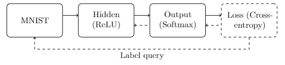
The first node (MNIST) will be responsible for acquiring new training samples and feeding it to the next layer for processing.
In addition, it will provide an accessor that the final categorical cross-entropy loss node will use to query the correct label for that sample (the “label query”).
The hidden node will perform the affine transform and apply the linear rectification activation.
The output node will also perform an affine transform, but will then apply the softmax function.
Finally, the loss node will compute the loss of the predicted distribution based on the queried label for a given sample.
In the figure above, solid arrows from left to right indicate data flow during the feedforward or evaluation portion of the model’s execution. Each solid arrow corresponds to a data vector emitted by the source, and ingested by the destination. The dashed arrows from right to left indicate data flow during the backpropagation or reverse accumulation portion of the algorithm. These arrows correspond to gradient vectors of the evaluated loss with respect to the outputs passed during the feedforward phase. For example, as seen above, the hidden node is expected to forward data to the output node ($\mathbf{a}^{[1]}$). Later, after the model prediction has been computed and the loss evaluated, the gradient of the loss with respect to those outputs is expected ($\partial J_{CE}/\partial a^{[1]}_i$ for each $a_i^{[1]}$ in $\mathbf{a}^{[1]}$).
When simply evaluating the model (without training), the final loss node will simply be omitted from the graph. In addition, no back-propagation of gradients will occur as the model parameters are ossified during evaluation.
The model class interface shown below will be used to house all the nodes in the computational graph, and provide various routines that are useful for operating over all constituent nodes as a collection.
class Model
{
public:
    Model(std::string name);

    // Add a node to the model, forwarding arguments to the node's constructor
    template <typename Node_t, typename... T>
    Node_t& add_node(T&&... args)
    {
        nodes_.emplace_back(
            std::make_unique<Node_t>(*this, std::forward<T>(args)...));
        return reinterpret_cast<Node_t&>(*nodes_.back());
    }

    // Create a dependency between two constituent nodes
    void create_edge(Node& dst, Node& src);

    // Initialize the parameters of all nodes with the provided seed. If the
    // seed is 0, a new random seed is chosen instead. Returns the seed used.
    rne_t::result_type init(rne_t::result_type seed = 0);

    // Adjust all model parameters of constituent nodes using the
    // provided optimizer (shown later)
    void train(Optimizer& optimizer);

    std::string const& name() const noexcept
    {
        return name_;
    }

    void print() const;

    // Routines for saving and loading model parameters to and from disk
    void save(std::ofstream& out);
    void load(std::ifstream& in);

private:
    friend class Node;

    std::string name_;
    std::vector<std::unique_ptr<Node>> nodes_;
};
Training Data and Labels
All machine learning pipelines must consider how to ingest data and labels.
Data refers to the information the model is expected to use to make inferences and predictions.
Labels correspond to the “correct answer” for each data sample, used to compute losses and train the model.
The interface of the MNIST data parser is shows below as an implemented Node class.
class MNIST : public Node
{
public:
    constexpr static size_t DIM = 28 * 28;

    // The constructor receives an input filestream corresponding to the
    // data samples and labels
    MNIST(Model& model, std::ifstream& images, std::ifstream& labels);

    // This is an input node and has no parameters to initialize
    void init(rne_t&) override {}

    // Read the next sample and label and forward the data
    void forward(num_t* data = nullptr) override;

    // No optimization is done in this node so this is a no-op
    void reverse(num_t* gradients = nullptr) override {}

    void print() const override;

    // Consume the next sample and label from the file streams
    void read_next();

    // Accessor for the most recently read sample
    num_t const* data() const noexcept
    {
        return data_;
    }

    // Accessor for the most recently read label
    num_t* label() const noexcept
    {
        return label_;
    }

    // Quick ASCII visualization of the last digit read
    void print_last();

private:
    std::ifstream& images_;
    std::ifstream& labels_;
    uint32_t image_count_;

    char buf_[DIM];
    num_t data_[DIM];
    num_t label_[10];
};
In the constructor, we must verify that the files passed as arguments are valid MNIST data and label files. Both files start with distinct “magic values” as a quick sanity check. The sample file starts with 2051 encoded as a 4-byte big-endian unsigned integer, whereas the label file starts with 2049. For the data file, the magic number is followed by the image count and image dimensions. The label file magic number is followed by the label count (expected to match the image count).
To consume big-endian unsigned integers from the file stream, we’ll use a simple routine:
void read_be(std::ifstream& in, uint32_t* out)
{
    char* buf = reinterpret_cast<char*>(out);
    in.read(buf, 4);

    std::swap(buf[0], buf[3]);
    std::swap(buf[1], buf[2]);
}
If you happen to be using a big-endian processor, you will not need to perform the byte swaps, but most desktop and mobile architectures are little-endian.
The implementation that parses the magic numbers and various other descriptors is produced below:
MNIST::MNIST(Model& model, std::ifstream& images, std::ifstream& labels)
    : Node{model, "MNIST input"}
    , images_{images}
    , labels_{labels}
{
    // Confirm that passed input file streams are well-formed MNIST data sets
    uint32_t image_magic;
    read_be(images, &image_magic);
    if (image_magic != 2051)
    {
        throw std::runtime_error{"Images file appears to be malformed"};
    }
    read_be(images, &image_count_);

    uint32_t labels_magic;
    read_be(labels, &labels_magic);
    if (labels_magic != 2049)
    {
        throw std::runtime_error{"Labels file appears to be malformed"};
    }

    uint32_t label_count;
    read_be(labels, &label_count);
    if (label_count != image_count_)
    {
        throw std::runtime_error(
            "Label count did not match the number of images supplied");
    }

    uint32_t rows;
    uint32_t columns;
    read_be(images, &rows);
    read_be(images, &columns);
    if (rows != 28 || columns != 28)
    {
        throw std::runtime_error{
            "Expected 28x28 images, non-MNIST data supplied"};
    }

    printf("Loaded images file with %d entries\n", image_count_);
}
Next, let’s implement the MNIST::read_next, which will consume the next
sample and label from the file streams:
void MNIST::read_next()
{
    images_.read(buf_, DIM);
    num_t inv = num_t{1.0} / num_t{255.0};
    for (size_t i = 0; i != DIM; ++i)
    {
        data_[i] = static_cast<uint8_t>(buf_[i]) * inv;
    }

    char label;
    labels_.read(&label, 1);

    for (size_t i = 0; i != 10; ++i)
    {
        label_[i] = num_t{0.0};
    }
    label_[static_cast<uint8_t>(label)] = num_t{1.0};
}
For the labels, note that the label is encoded as a single unsigned digit, but we convert it to a 1-hot encoding for loss computation purposes later. If your application can assume that the labels will be one-hot encoded, this conversion may not be necessary and a more efficient implementation is possible.
To verify our work, let’s write up a quick-and-dirty ASCII printer for the last read digit and try our parser out. If you have a rendering backend (written in say, Vulkan, D3D12, OpenGL, etc.) at your disposal, you may wish to use that instead for a cleaner visualization.
void MNIST::print_last()
{
    for (size_t i = 0; i != 10; ++i)
    {
        if (label_[i] == num_t{1.0})
        {
            printf("This is a %zu:\n", i);
            break;
        }
    }

    for (size_t i = 0; i != 28; ++i)
    {
        size_t offset = i * 28;
        for (size_t j = 0; j != 28; ++j)
        {
            if (data_[offset + j] > num_t{0.5})
            {
                if (data_[offset + j] > num_t{0.9})
                {
                    printf("#");
                }
                else if (data_[offset + j] > num_t{0.7})
                {
                    printf("*");
                }
                else
                {
                    printf(".");
                }
            }
            else
            {
                printf(" ");
            }
        }
        printf("\n");
    }
    printf("\n");
}
On my machine, consuming the evaluation data and printing it produces the following result (the first sample from the test data is shown):
This is a 7:

       *..
      *#####********.
          .*#*####*##.
                   ##
                   #*
                  ##
                 .##
                 ##
                .#*
                *#
                #*
               ##
              *#.
             *#*
             ##
            *#
           .##
           ###
           ##*
           #*
so we can be somewhat confident that our MNIST data ingestor is working properly. The only
remaining routine we need to implement is MNIST::forward which should consume the
next sample, and forward the data to all subsequent nodes in the graph.
void MNIST::forward(num_t* data)
{
    read_next();
    for (Node* node : subsequents_)
    {
        node->forward(data_);
    }
}
Such an interface ensures our MNIST node will be interoperable with networks
that aren’t purely sequential.
The Feedforward Node
The hidden and output nodes have much in common and so will be implemented in terms of
a single feedforward node class. The feedforward node will need a configurable activation
function and dimensionality. Here’s the interface for the FFNode:
enum class Activation
{
    ReLU,
    Softmax
};

class FFNode : public Node
{
public:
    // A feedforward node is defined by the activation
    // function and input/output dimensionality
    FFNode(Model& model,
           std::string name,
           Activation activation,
           uint16_t output_size,
           uint16_t input_size);

    void init(rne_t& rne) override;

    // The input data should have size input_size_
    void forward(num_t* inputs) override;

    // The gradient data should have size output_size_
    void reverse(num_t* gradients) override;

    size_t param_count() const noexcept override
    {
        // Weight matrix entries + bias entries
        return (input_size_ + 1) * output_size_;
    }

    num_t* param(size_t index);
    num_t* gradient(size_t index);

    void print() const override;

private:
    Activation activation_;
    uint16_t output_size_;
    uint16_t input_size_;

    /////////////////////
    // Node Parameters //
    /////////////////////

    // weights_.size() := output_size_ * input_size_
    std::vector<num_t> weights_;
    // biases_.size() := output_size_
    std::vector<num_t> biases_;
    // activations_.size() := output_size_
    std::vector<num_t> activations_;

    ////////////////////
    // Loss Gradients //
    ////////////////////

    std::vector<num_t> activation_gradients_;

    // During the training cycle, parameter loss gradients are accumulated in
    // the following buffers.
    std::vector<num_t> weight_gradients_;
    std::vector<num_t> bias_gradients_;

    // This buffer is used to store temporary gradients used in a SINGLE
    // backpropagation pass. Note that this does not accumulate like the weight
    // and bias gradients do.
    std::vector<num_t> input_gradients_;

    // The last input is needed to compute loss gradients with respect to the
    // weights during backpropagation
    num_t* last_input_;
};
Compared to the MNIST node, the FFNode uses a lot more state to track
all tunable parameters (weight matrix elements and biases), as well as the
loss gradients corresponding to each parameter. The loss gradients must
be kept because, remember, utilizing them to actually adjust the parameters
is performed only after N samples have been evaluated, where N is the
chosen batch size in our stochastic gradient descent algorithm. If the
purpose of some of the class members here is still opaque, they will show up
later when implement backpropagation.
First, we must decide how to initialize the weights and biases of our node. When deciding on a scheme, there are a few key principles to keep in mind. First, the initialization must exhibit symmetry of any sort. For example, if all the parameters are initialized to the same random value, the loss gradients with respect to all individual parameters will be identical, and our network will be no better than a network with a single parameter. In addition, we do not want the parameters to be initialized such that they are too large, or too small. Most papers that discuss weight initialization strive to ensure that the loss gradients remain in a realm where floating point number retain precision (in the range $[1, 2)$). The other criteria is that parameters should generally be initialized such that they are roughly similar in magnitude. Parameters that deviate too far from the mean are likely to either dominate loss gradients, or produce too small a signal to contribute. Proper parameter initialization is but a small part of addressing the larger problem common in neural networks known as the problem of exploding and vanishing gradients. Here, we present the implementation with a couple references if you wish to dig deeper.
void FFNode::init(rne_t& rne)
{
    num_t sigma;
    switch (activation_)
    {
    case Activation::ReLU:
        // Kaiming He, et. al. weight initialization for ReLU networks
        // https://arxiv.org/pdf/1502.01852.pdf
        //
        // Suggests using a normal distribution with variance := 2 / n_in
        sigma = std::sqrt(2.0 / static_cast<num_t>(input_size_));
        break;
    case Activation::Softmax:
    default:
        // LeCun initialization as suggested in "Self-Normalizing Neural
        // Networks"
        // https://arxiv.org/pdf/1706.02515.pdf
        sigma = std::sqrt(1.0 / static_cast<num_t>(input_size_));
        break;
    }

    // NOTE: Unfortunately, the C++ standard does not guarantee that the results
    // obtained from a distribution function will be identical given the same
    // inputs across different compilers and platforms. A production ML
    // framework will likely implement its own distributions to provide
    // deterministic results.
    auto dist = std::normal_distribution<num_t>{0.0, sigma};

    for (num_t& w : weights_)
    {
        w = dist(rne);
    }

    // NOTE: Setting biases to zero is a common practice, as is initializing the
    // bias to a small value (e.g. on the order of 0.01). It is unclear if the
    // latter produces a consistent result over the former, but the thinking is
    // that a non-zero bias will ensure that the neuron always "fires" at the
    // beginning to produce a signal.
    //
    // Here, we initialize all biases to a small number, but the reader should
    // consider experimenting with other approaches.
    for (num_t& b : biases_)
    {
        b = 0.01;
    }
}
The common theme is that the distribution of random weights scales roughly as the inverse square root of the input vector size. This way, the distribution of the node’s output will fall in a “nice” range with respect to floating-point precision. Other initialization schemes are of course possible, and in some cases critical depending on the choice of activation function.
With weights and biases initialized, it’s time to implement FFNode::forward.
The straightforward plan is, for both the ReLU and softmax nodes, first perform the
affine transform $\mathbf{W}\mathbf{x} + \mathbf{b}$, then perform the activation function
which will be one of the linear rectifier or the softmax function. Here’s what this
looks like:
void FFNode::forward(num_t* inputs)
{
    // Remember the last input data for backpropagation later
    last_input_ = inputs;

    for (size_t i = 0; i != output_size_; ++i)
    {
        // For each output vector, compute the dot product of the input data
        // with the weight vector add the bias

        num_t z{0.0};

        size_t offset = i * input_size_;

        for (size_t j = 0; j != input_size_; ++j)
        {
            z += weights_[offset + j] * inputs[j];
        }
        // Add neuron bias
        z += biases_[i];

        switch (activation_)
        {
        case Activation::ReLU:
            activations_[i] = std::max(z, num_t{0.0});
            break;
        case Activation::Softmax:
        default:
            activations_[i] = std::exp(z);
            break;
        }
    }

    if (activation_ == Activation::Softmax)
    {
        // softmax(z)_i = exp(z_i) / \sum_j(exp(z_j))
        num_t sum_exp_z{0.0};
        for (size_t i = 0; i != output_size_; ++i)
        {
            // NOTE: with exploding gradients, it is quite easy for this
            // exponential function to overflow, which will result in NaNs
            // infecting the network.
            sum_exp_z += activations_[i];
        }
        num_t inv_sum_exp_z = num_t{1.0} / sum_exp_z;
        for (size_t i = 0; i != output_size_; ++i)
        {
            activations_[i] *= inv_sum_exp_z;
        }
    }

    // Forward activation data to all subsequent nodes in the computational
    // graph
    for (Node* subsequent : subsequents_)
    {
        subsequent->forward(activations_.data());
    }
}
As before, we forward all final results to all subsequent nodes even though there will only be a single subsequent node in this case. Whenever writing code as above, it is prudent to consider all potential corner cases which could result in the myriad issues that arise in floating-point computation:
- Loss of precision
- Floating point overflow and underflow
- Divide by zero
Loss of precision easily occurs when in a number of situations, such as subtracting
two quantities of similar size, or adding and multiplying quantities with
greatly different magnitudes. Floating point overflow and underflow occur
typically when repeatedly performing an operation such that an accumulator explodes
to $\infty$ or $-\infty$. In this case, the use of std::exp is one operation
that sticks out. We will not implement a stable softmax here, but the following identity
can be used to improve its stability should you need it:
In this expression, $\mathbf{C}$ is a constant vector where all its elements are equal in value. Expanding the definition of softmax in the LHS gives:
\[\begin{aligned} \mathrm{softmax}(\mathbf{z} + \mathbf{C})_i &= \frac{\exp{(z_i + C)}}{\sum_i\exp{(z_i + C})} \\ &= \frac {\exp{z_i}\exp{C}} {\left(\sum_i\exp{z_i}\right)\exp C} \\ &= \mathrm{softmax}(\mathbf{z})_i && \blacksquare \end{aligned}\]Thus, if we are considered about saturating std::exp with a large argument, we can simply set
$C$ to be the additive inverse of the $z_i$ with the greatest magnitude within $\mathbf{z}$. Performing this
each time we apply softmax will usually maintain the arguments of the softmax within a reasonable
range (unless elements of $z_i$ explode in opposite directions).
As a practical implementor’s trick, it is possible to enable floating point exception traps
to throw an exception when a NaN is generated in a floating point register. Using libc
for example, we can trap floating point exceptions using
#include <cfenv>

feenableexcept(FE_INVALID | FE_OVERFLOW);
It is also possible to trap exceptions specifically in regions where you anticipate a potential issue (which enhances the overall throughput of the network). In the interest of brevity, please consult your compiler’s documentation for how to do this.
One observation you might have made is the first line of our routine.
last_input_ = inputs;
Here, we retain a pointer to the data ingested by the feedforward node for a full training cycle. Before delving into any derivations, let’s first present the code for the backpropagation of gradients through our feedforward node and dissect it immediately afterwards.
void FFNode::reverse(num_t* gradients)
{
    // First, we compute dJ/dz as dJ/dg(z) * dg(z)/dz and store it in our
    // activations array
    for (size_t i = 0; i != output_size_; ++i)
    {
        // dg(z)/dz
        num_t activation_grad{0.0};
        switch (activation_)
        {
        case Activation::ReLU:
            if (activations_[i] > num_t{0.0})
            {
                activation_grad = num_t{1.0};
            }
            else
            {
                activation_grad = num_t{0.0};
            }
            // dJ/dz = dJ/dg(z) * dg(z)/dz
            activation_gradients_[i] = gradients[i] * activation_grad;
            break;
        case Activation::Softmax:
        default:
            for (size_t j = 0; j != output_size_; ++j)
            {
                if (i == j)
                {
                    activation_grad += activations_[i]
                                       * (num_t{1.0} - activations_[i])
                                       * gradients[j];
                }
                else
                {
                    activation_grad
                        += -activations_[i] * activations_[j] * gradients[j];
                }
            }

            activation_gradients_[i] = activation_grad;
            break;
        }
    }

    for (size_t i = 0; i != output_size_; ++i)
    {
        // dJ/db_i = dJ/dg(z_i) * dJ(g_i)/dz_i.
        bias_gradients_[i] += activation_gradients_[i];
    }

    std::fill(input_gradients_.begin(), input_gradients_.end(), 0);

    for (size_t i = 0; i != output_size_; ++i)
    {
        size_t offset = i * input_size_;
        for (size_t j = 0; j != input_size_; ++j)
        {
            input_gradients_[j]
                += weights_[offset + j] * activation_gradients_[i];
        }
    }

    for (size_t i = 0; i != input_size_; ++i)
    {
        for (size_t j = 0; j != output_size_; ++j)
        {
            weight_gradients_[j * input_size_ + i]
                += last_input_[i] * activation_gradients_[j];
        }
    }

    for (Node* node : antecedents_)
    {
        node->reverse(input_gradients_.data());
    }
}
This code is likely more difficult to digest, so let’s break it down into parts. During reverse accumulation (aka backpropagation), we will be given the loss gradients with respect to all of the outputs from the most recent forward pass, written mathematically as $\partial J_{CE}/\partial a_i$ for each output scalar $a_i$. Given that information, we need to perform the following tasks:
- Compute $\partial J_{CE}/\partial w_{ij}$ for each weight in our weight matrix
- Compute $\partial J_{CE}/\partial b_i$ for each bias in our bias vector
- Compute $\partial J_{CE}/\partial x_i$ for each input scalar in the most recent forward pass
- Propagate all the loss gradients with respect to the inputs in step 3 back to the antecedent nodes
As all outputs pass through an activation function, we will need to compute
\[\frac{\partial J_{CE}}{\partial g(\mathbf{z})_i}\]where $g$ is one of the linear rectifier or softmax function corresponding to a particular component of the output vector. Both derivatives are computed in the background section, so we’ll just recite the results here. For the linear rectifier, $\partial J_{CE}/\partial g(\mathbf{z})_i$ will simply be 1 if $a_i \neq 0$, and 0 otherwise. The softmax gradient is slightly more involved, but because every output of the softmax contributes additively to the loss, we require a sum of gradients here:
\[\frac{\partial J_{CE}}{\partial \mathrm{softmax}(\mathbf{z})_i} = \frac{\partial J_{CE}}{\partial a_i}\sum_{j} \begin{cases} \mathrm{softmax}(\mathbf{z})_i\left(1 - \mathrm{softmax}(\mathbf{z})_i\right) & i = j \\ -\mathrm{softmax}(\mathbf{z})_i \mathrm{softmax}(\mathbf{z})_j & i \neq j \end{cases}\]The factor $\partial J_{CE}/\partial a_i$ comes from the chain rule and is passed in from the subsequent node.
These intermediate expressions are computed, scaled by $\partial a_i/\partial z_i$, and then stored in activation_gradients_ in the top portion
of FFNode::reverse.
Equivalently by the chain rule, we are caching in activation_gradients_ $\partial J_{CE}/\partial z_i$ for each $i$.
Because the loss gradients with respect to every parameter and input have a functional dependence on the activation function
gradients, all results computed in tasks 1 through 4 above will depend on activation_gradients_.
Computing bias gradients
The bias gradients are the easiest to compute due to how they show up in the expression. Since a node’s output is given as
\[a_i = g\left(\mathbf{W}_i \cdot \mathbf{x} + b_i = z_i\right)\]for some activation function $g$, the derivative with respect to $b_i$ is just
\[\begin{aligned} \frac{\partial{a_i}}{\partial b_i} &= \frac{\partial g}{\partial z_i}\frac{\partial z_i}{\partial b_i} \\ &= \frac{\partial g}{\partial z_i} \end{aligned}\]Thus we can simply accumulate the result stored in activation_gradients_ as the loss gradient with
respect to each bias. Please take note! The code that performs this update is
    for (size_t i = 0; i != output_size_; ++i)
    {
        bias_gradients_[i] += activation_gradients_[i];
    }
The following code would not be correct:
    for (size_t i = 0; i != output_size_; ++i)
    {
        // NOTE: WRONG! Will only alone batch sizes of 1
        bias_gradients_[i] = activation_gradients_[i];
    }
As the admonition in the comment suggests, while it’s helpful to conceptualize the loss gradient as something that resets every time we perform a forward and reverse pass of a training sample, in actuality, we require the gradients with respect to the cumulative mean loss accrued while evaluating the entire batch for stochastic gradient descent. Luckily, because the losses per sample accumulate additively, the gradients of the loss with respect to all parameters in the model also update additively.
Computing the weight gradients
The weight gradients are slightly more involved than the bias gradients, but are still relatively easy to compute with a bit of bookkeeping. For any given weight $w_{ij}$, we can observe that such a weight participates only in the evaluation of $z_i$. That is:
\[\begin{aligned} \frac{\partial \mathbf{z}}{\partial w_{ij}} &= \frac{\partial z_i}{\partial w_{ij}} \\ &= \frac{\partial (\mathbf{w}_{i} \cdot \mathbf{x}) + b_i}{\partial w_{ij}} \\ &= x_j \\ \end{aligned}\] \[\boxed{\frac{\partial J_{CE}}{\partial w_{ij}} = \frac{\partial J_{CE}}{\partial a_i}\frac{\partial a_i}{\partial z_i}x_j}\]The boxed result shows the final loss gradient with respect to a weight parameter. The weight gradient accumulation appears in the following code, where all $N \times M$ weights are updated in a couple of nested loops:
    for (size_t i = 0; i != input_size_; ++i)
    {
        for (size_t j = 0; j != output_size_; ++j)
        {
            weight_gradients_[j * input_size_ + i]
                += last_input_[i] * activation_gradients_[j];
        }
    }
Computing the input gradients
The last set of gradients we need to compute are the loss gradients with respect to the inputs, to be forwarded to the antecedent node. This calculation is similar to the calculation of the weight gradients in terms of the linear dependence. However, it is important to note that a given input participates in the computation of all output scalars. Thus, we expect each individual input gradient to be a summation.
\[\frac{\partial J_{CE}}{\partial x_i} = \sum_j \frac{\partial J_{CE}}{\partial a_j}\frac{\partial a_j}{\partial z_j}w_{ij}\]The code that computes the input gradients is defined here:
    std::fill(input_gradients_.begin(), input_gradients_.end(), 0);

    for (size_t i = 0; i != output_size_; ++i)
    {
        size_t offset = i * input_size_;
        for (size_t j = 0; j != input_size_; ++j)
        {
            input_gradients_[j]
                += weights_[offset + j] * activation_gradients_[i];
        }
    }
Note that unlike the weight and bias gradients which accumulate while training an entire batch of samples, the input gradients here are ephemeral and reset every pass since the only depend on the evaluation of an individual sample.
Finally, to complete the FFNode::reverse method, the input gradients computed
are based backwards for use in an antecedent node’s gradient update (reproduced below). The code as
presented does not work with non-sequential computational graphs, but is meant
to provide a starting point for futher experimentation.
    for (Node* node : antecedents_)
    {
        node->reverse(input_gradients_.data());
    }
The Categorical Cross-Entropy Loss Node
The last node we need to implement is the node which computes the categorical cross-entropy of the prediction. A possible class definition for such this node is shown below:
class CCELossNode : public Node
{
public:
    CCELossNode(Model& model,
                std::string name,
                uint16_t input_size,
                size_t batch_size);

    // No initialization is needed for this node
    void init(rne_t&) override {}

    void forward(num_t* inputs) override;

    // As a loss node, the argument to this method is ignored (the gradient of
    // the loss with respect to itself is unity)
    void reverse(num_t* gradients = nullptr) override;

    void print() const override;

    // During training, this must be set to the expected target distribution
    // for a given sample
    void set_target(num_t const* target)
    {
        target_ = target;
    }

    num_t accuracy() const;
    num_t avg_loss() const;
    void reset_score();

private:
    uint16_t input_size_;

    // We minimize the average loss, not the net loss so that the losses
    // produced do not scale with batch size (which allows us to keep training
    // parameters constant)
    num_t inv_batch_size_;
    num_t loss_;
    num_t const* target_;
    num_t* last_input_;
    // Stores the last active classification in the target one-hot encoding
    size_t active_;
    num_t cumulative_loss_{0.0};
    // Store running counts of correct and incorrect predictions
    size_t correct_   = 0;
    size_t incorrect_ = 0;
    std::vector<num_t> gradients_;
};
The CCELossNode is similar to other nodes in that it implements a forward pass
for computing the loss of a given sample, and a reverse pass to compute gradients
of that loss and pass them back to the antecedent node. Distinct from the previous
nodes is that the argument to CCELossNode::reverse is ignored as the loss node
is not expected to have any subsequents.
The implementation of CCELossNode::forward follows from the definition of cross-entropy,
recalled here with some modifications:
$J$ is the common symbol ascribed to the cost or objective function, while $\hat{y}$ and $y$ refer to the predicted distribution and correct distribution respectively. In addition, the argument of the logarithm is clamped with a small $\epsilon$ to avoid a numerical singularity. The implementation is as follows:
void CCELossNode::forward(num_t* data)
{
    num_t max{0.0};
    size_t max_index;

    loss_ = num_t{0.0};
    for (size_t i = 0; i != input_size_; ++i)
    {
        if (data[i] > max)
        {
            max_index = i;
            max       = data[i];
        }

        loss_ -= target_[i]
                 * std::log(
                     std::max(data[i], std::numeric_limits<num_t>::epsilon()));

        if (target_[i] != num_t{0.0})
        {
            active_ = i;
        }
    }

    if (max_index == active_)
    {
        ++correct_;
    }
    else
    {
        ++incorrect_;
    }

    cumulative_loss_ += loss_;

    // Store the data pointer to compute gradients later
    last_input_ = data;
}
As with the feedforward node, a pointer to the inputs to the node is preserved to compute gradients later. A bit of bookkeeping is also done so we can track accuracy and accumulate loss during batch. The derivative of the loss of an individual sample with respect to the inputs is also fairly straightforward.
\[\begin{aligned} \frac{\partial J_{CE}}{\partial{\hat{y}_i}} &= \frac{\partial \left(-\sum_j y_j\log{\left(\max(\hat{y}_j, \epsilon)\right)}\right)}{\partial \hat{y}_i} \\ &= -\frac{y_i}{\max(\hat{y}_i, \epsilon)} \end{aligned}\]The implementation is similarly straightforward. As with the other nodes with loss gradients, the loss gradients with respect to all inputs are forwarded to antecedent nodes.
void CCELossNode::reverse(num_t* data)
{
    for (size_t i = 0; i != input_size_; ++i)
    {
        gradients_[i] = -inv_batch_size_ * target_[i]
            / std::max(last_input_[i], std::numeric_limits<num_t>::epsilon());
    }

    for (Node* node : antecedents_)
    {
        node->reverse(gradients_.data());
    }
}
One thing to keep in mind here is that this implementation is not the most efficient implementation possible for a softmax layer feeding to a cross-entropy loss function by any stretch. The code and derivation here is completely general for arbitrary sample probability distributions. If, however, we can assume that the target distribution is one-hot encoded, then all gradients in this node will either be 0 or $-1/\hat{y}_k$ where $k$ is the active label in the one-hot target. Upon substitution in the previous layer, it should be clear that important cancellations are possible that dramatically simplify the gradient computations in the softmax layer. Here’s the simplification, again assuming that the $k$th index is the correct label:
\[\begin{aligned} \frac{\partial J_{CE}}{\partial \mathrm{softmax}(\mathbf{z})_i} &= \frac{\partial J_{CE}}{\partial a_i}\sum_{j} \begin{cases} \mathrm{softmax}(\mathbf{z})_i\left(1 - \mathrm{softmax}(\mathbf{z})_i\right) & i = j \\ -\mathrm{softmax}(\mathbf{z})_i \mathrm{softmax}(\mathbf{z})_j & i \neq j \end{cases} \\ &= \begin{dcases} -\frac{\mathrm{softmax}(\mathbf{z})_k(1 - \mathrm{softmax}(\mathbf{z}_k))}{\mathrm{softmax}(\mathbf{z})_k} & i = k \\ \frac{\mathrm{softmax}(\mathbf{z})_i\mathrm{softmax}(\mathbf{z})_k}{\mathrm{softmax}(\mathbf{z})_k} & i \neq k\\ \end{dcases} \\ &= \begin{dcases} \mathrm{softmax}(\mathbf{z})_k - 1 & i = k \\ \mathrm{softmax}(\mathbf{z})_i & i \neq k \end{dcases} \end{aligned}\]When following the computation above, remember that $\partial J_{CE} / \partial a_i$ is 0 for all $i \neq k$. Thus, the only term in the sum that survives is the term corresponding to $j = k$, at which point we break out the differentation depending on whether $i = k$ or $i \neq k$.
This is an elegant result! Essentially, the gradient of a the loss with respect to an emitted probability $p(x)$ is simply $p(x)$ if $x$ was not the correct label, and $p(x) - 1$ if it was. Considering the effect of gradient descent, this should check out with our intuition. The optimizer seeks to suppress probabilities predicted that should have been 0, and increase probabilities predicted that should have been 1. Check for yourself that after gradient descent is performed, the gradients derived here will nudge the model in the appropriate direction.
This sort of optimization highlights an important observation about backpropagation, namely, that backpropagation does not guarantee any sort of optimality beyond a worst-case performance ceiling. Several production neural networks have architectures that employ heuristics to identify optimizations such as this one, but the problem of generating a perfect computational strategy is NP and so not covered here. The code provided here will remain in the general form, despite being slower in the interest of maintaining generality and not adding complexity, but you are encouraged to consider abstractions to permit this type of optimization in your own architecture (a useful keyword to aid your research is common subexpression elimination or CSE for short).
The last thing we need to provide for CCELossNode are a few helper routines:
void CCELossNode::print() const
{
    std::printf("Avg Loss: %f\t%f%% correct\n", avg_loss(), accuracy() * 100.0);
}

num_t CCELossNode::accuracy() const
{
    return static_cast<num_t>(correct_)
           / static_cast<num_t>(correct_ + incorrect_);
}
num_t CCELossNode::avg_loss() const
{
    return cumulative_loss_ / static_cast<num_t>(correct_ + incorrect_);
}

void CCELossNode::reset_score()
{
    cumulative_loss_ = num_t{0.0};
    correct_         = 0;
    incorrect_       = 0;
}
These routines let us observe the performance of our network during training in terms of both loss and accuracy.
Gradient Descent Optimizer
At some point after loss gradients with respect to model parameters have accumulated,
the gradients will need to be used to actually adjust the parameters themselves. This is provided
by the GDOptimizer class implemented as below:
class GDOptimizer : public Optimizer
{
public:
    // "Eta" is the commonly accepted character used to denote the learning
    // rate. Given a loss gradient dJ/dp for some parameter p, during gradient
    // descent, p will be adjusted such that p' = p - eta * dJ/dp.
    GDOptimizer(num_t eta) : eta_{eta} {}

    // This should be invoked at the end of each batch's evaluation. The
    // interface technically permits the use of different optimizers for
    // different segments of the computational graph.
    void train(Node& node) override;

private:
    num_t eta_;
};

void GDOptimizer::train(Node& node)
{
    size_t param_count = node.param_count();
    for (size_t i = 0; i != param_count; ++i)
    {
        num_t& param    = *node.param(i);
        num_t& gradient = *node.gradient(i);

        param = param - eta_ * gradient;

        // Reset the gradient which will be accumulated again in the next
        // training epoch
        gradient = num_t{0.0};
    }
}
Not shown is the Optimizer class interface which simply provides a virtual train method.
As you implement more sophisticated optimizers, you will find that more state may be needed
to perform necessary tasks (e.g. computing gradient moving averages). Also implicit in this
implementation is that our Node classes need to provide an indexing scheme for each parameter
as well as an accessor for the total number of parameters. For example, accessing the FFNode parameters
is a fairly simple matter:
num_t* FFNode::param(size_t index)
{
    if (index < weights_.size())
    {
        return &weights_[index];
    }
    return &biases_[index - weights_.size()];
}
The parameters are indexed 0 through the return value of Node::param_count() minus one.
Note that the optimizer doesn’t care whether the parameter accessed in this way is a weight, bias, average, etc.
As a trainable parameter, the only thing that matters during gradient descent is the current value
and the loss gradient.
Tying it all Together
Now that we have the individual nodes implemented, all that remains is to wire things up and start training! This is how we can construct a model with a input, hidden, output, and loss nodes, all wired sequentially.
    Model model{"ff"};

    MNIST& mnist = &model.add_node<MNIST>(images, labels);

    FFNode& hidden = model.add_node<FFNode>("hidden", Activation::ReLU, 32, 784);

    FFNode& output
        = model.add_node<FFNode>("output", Activation::Softmax, 10, 32);

    CCELossNode& loss = &model.add_node<CCELossNode>("loss", 10, batch_size);
    loss.set_target(mnist.label());

    model.create_edge(hidden, mnist);
    model.create_edge(output, hidden);
    model.create_edge(loss, output);

    // This function should visit all constituent nodes and initialize
    // their parameters
    model.init();

    // Create a gradient descent optimizer with a hardcoded learning rate
    GDOptimizer optimizer{num_t{0.3}};
As mentioned before, the “edges” are somewhat cosmetic as none of our nodes actually support multiple node inputs or outputs. An actual implementation that would support such a non-sequential topology will likely need a sort of signals and slots abstraction. The interface provided here is strictly to impress on you the importance of the abstraction of our neural network as a computational graph, which is critical when additional complexity is added later.
With this, we are ready to implement the core loop of the training algorithm.
    for (size_t i = 0; i != 256; ++i)
    {
        for (size_t j = 0; j != 64; ++j)
        {
            mnist->forward();
            loss->reverse();
        }

        model.train(optimizer);
    }
Here, we train our model over 256 batches. Each batch consists of 64 samples, and for each
sample, we invoke MNIST::forward and CCELossNode::reverse. During the forward pass,
our MNIST node extracts a new sample and label and forwards the sample data to the next node.
This data propagates through the network until the final output distribution is passed to the
loss node and losses are computed. All this occurs within the single line: mnist->forward().
In the subsequent line, gradients are computed and passed back until the reverse accumulation
terminates at the MNIST node again. After all gradients for the batch are accumulated, the
model can train, which invokes the optimizer on each node to simultaneously adjust all
model parameters for each node.
After adding some additional logging, the results of the network look like this:
Executing training routine
Loaded images file with 60000 entries
hidden: 784 -> 32
output: 32 -> 10
Initializing model parameters with seed: 116726080
Avg Loss: 0.254111	96.875000% correct
To evaluate the efficacy of the model, we can serialize all the parameters to disk, load them up, disable the training step, and evaluate the model on the test data. For this particular run, the results were as follows:
Executing evaluation routine
Loaded images file with 10000 entries
hidden: 784 -> 32
output: 32 -> 10
Avg Loss: 0.292608	91.009998% correct
As you can see, the accuracy dropped on the test data relative to the training data. This is a hallmark characterstic of overfitting, which is to be expected given that we haven’t implemented any regularization whatsoever! That said, 91% accuracy isn’t all that bad when we consider the fact that our model has no notion of pixel-adjacency whatsoever. For image data, convolutional networks are a far more apt architecture than the one chosen for this demonstration.
Regularization
Regularization will not be implemented as part of this self-contained neural network, but it is such a fundamental part of most deep learning frameworks that we’ll discuss it here.
Often, the dimensionality of our model will be much higher than what is stricly needed to make accurate predictions. This stems from the fact that we seldom no a priori how many features are needed for the model to be successful. Thus, the likelihood of overfitting increases as more training data is fed into the model. The primary tool to combat overfitting is regularization. Loosely speaking, regularization is any strategy employed to restrict the hypothesis space of fit-functions the model can occcupy to prevent overfitting.
What is meant by restricting the hypothesis space, you might ask? The idea is to consider the entire family of functions possible spanned by the model’s entire parameter vector. If our model has 10000 parameters (many networks will easily exceed this), each unique 10000-dimensional vector corresponds to a possible solution. However, we know it’s unlikely that certain parameters should be vastly greater in magnitude than others in a theoretically optimal condition. Models with “strange” parameter vectors that are unlikely to be the optimal solution are likely converged on as a result of overfitting. Therefore, it makes sense to consider ways to constrain the space this parameter vector may occupy.
The most common approach to achieve this is to add an initial penalty term to the loss function which is a function of the weight. For example, here is the cross-entropy loss with the so-called $L^2$ regularizer (also known as the ridge regularizer) added:
\[-\sum_{x\in X} y_x \log{\hat{y}_x} + \frac{\lambda}{2} \mathbf{w}^{T}\mathbf{w}\]In a slight abuse of notation, $\mathbf{w}$ here corresponds to a vector containing every weight in our network. The factor $\lambda$ is a constant we can choose to adjust the penalty size. Note that when a regularizer is used, we expect training loss to increase. The tradeoff is that we simultaneously expect test loss to decrease. Tuning the regularization speed $\lambda$ is a routine problem for model fitting in the wild.
By modifying the loss function, in principal, all loss gradients must change as well. Fortunately, as we’ve only added a quadratic term to the loss, the only change to the gradient will be an additional linear additive term $\lambda\mathbf{w}$. This means we don’t have to add a ton of code to modify all the gradient calculations thus far. Instead, we can simply decay the weight based on a percentage of the weight’s magnitude when we adjust the weight after each batch is performed. You will often here this type of regularization referred to as simply weight decay for this reason.
To implement $L^2$ regularization, simply add a percentage of a weight’s value to its loss gradient. Crucially, do not adjust bias parameters in the same way. We only wish to penalize parameters for which increased magnitude corresponds with more complex models. Bias parameters are simply scalar offsets, regardless of their value and do not scale the inputs. Thus, attempting to regularize them will likely increase both training and test error.
Where to go from here
At this point, our toy network is complete. With any luck, you’ve taken away a few key patterns that will aid in both your intuition about how deep learning techniques work, and your efforts to actually implement them. The implementation presented here is both far from complete, and far from ideal. Critically missing is adequate visualization for the error rate as a function of training time, mis-predicted samples, and the model parameters themselves. Without visualization, model tuning can be time consuming, veering on impossible. In addition, our model training samples are always ingested in the order they are provided in the training file. In practice, this sequence should be shuffled to avoid introducing training bias.
Here are a few additional things you can try, in no particular order.
- Add various regularization modes such as $L^2$, $L^1$, or dropout.
- Track loss reduction momentum to implement early stopping, thereby reducing wasted training cycles
- Implement a convolution node with a variable sized weight filter. You will likely need to implement the max-pooling operation as well.
- Implement a batch-normalization node.
- Modify the interfaces provided here so that
Node::forwardandNode::reversealso pass slot ids to handle nodes with multiple inputs and outputs. - Leverage the slots abstraction above to implement a residual network.
- Improve efficiency by adding support for SIMD or GPU-based compute kernels.
- Add multithreading to allow separate batches to be trained simultaneously.
- Provide alternative optimizers that decay the learning rate over time, or decay the learning rate as a function of loss momentum.
- Add a “meta-training” feature that can tune hyperparameters used to configure your model (e.g. learning rate, regularization rate, network depth, layer dimension).
- Pick a research paper you’re interested in and endeavor to implement it end to end.
As you can see, the sky’s the limit and there is simply no end to the amount of work possible to improve a neural network’s ability to learn and make inferences. A good body of work is also there to improve tooling around data ingestion, model configuration serialization, automated testing, continuous learning in the cloud, etc. Crucially though, new research and development is constantly in the works in this ever-changing field. On top of studying deep learning as a discipline in and of itself, there is plenty of room for specialization in particular domains, be it computer vision, NLP, epidemiology, or something else. My hope is that for some of you, the neural network in a weekend may take the form of a neural network in a fulfilling career or lifetime.
Further Reading
If you get a single book, Deep Learning (listed first in the following table) is highly recommended as a relatively self-complete text with cogent explanations written in a readable style. As you venture into attempting to perform ML tasks in a particular domain, search for a relatively recent highly cited “survey” paper, which should introduce you to the main ideas and give you a starting point for further research. Here is an example of one such survey paper, in this case with an emphasis on object detection.
| Title | Authors | Description |
|---|---|---|
| Deep Learning | Ian Goodfellow, Yoshua Bengio, and Aaron Courville | Seminal text on the theory and practice of using neural networks to learn and perform tasks |
| Numerical Methods for Scientists and Engineers | R. W. Hamming | Excellent general text covering important topics such as floating point precision and various approximation methods |
| Standard notations for Deep Learning (link) | Stanford CS230 Course Notes | Cheatsheet covering standard notation used by many texts and papers |
| Neural Networks and Deep Learning (link) | Michael Nielsen | A gentler introduction to the theory and practice of neural networks |
| Automatic Differentiation in Machine Learning: a Survey (link) | Atılım Güneş Baydin, Barak A. Pearlmutter, Alexey Andreyevich Radul, Jeffrey Mark Siskind | Excellent survey paper documentating the various algorithms used for computational differentiation including viable alternatives to backpropagation |