Graphics Pipelines for Young Bloods
Forward, deferred, and friends.
When I first started graphics programming, I thought about pixels and scanlines first, and later graduated to happily shading 3D geometry via vertex and fragment shaders (circa OpenGL 2.0 and DirectX9 days). It didn’t take us long, however, to grow to a veritable zoo of available techniques. You have forward and deferred, variants of each (tiled, tiled deferred, clustered, clustered deferred), sub-variants like deferred texturing, visibility buffers, and the list goes on. For graphics programmers that didn’t have a benefit of learning these various pipelines as they emerged, this article is for you. Especially with yet more tools in our toolbox (mesh/amplification shaders, hardware raytracing, compute capabilities, etc), it’s important to understand the underlying principles before trying to grok the hyper-modern AAA pipeline.
Namely, what are we trading off when we opt to render or light an object with one pipeline vs another? Understanding how to analyze a pipeline through this lens is critical to appreciating the spectrum of rendering techniques at our disposal, and finding the set of tradeoffs that’s right for each of your use cases. The primary audience for this post is the set of newer graphics programmers (say, less than 3 years of experience) or programmers that have worked with traditional pipelines and want to get up to speed on changes in, say, the last 10 years or so.
TL; DR The bulk of this post will mainly discuss the various tradeoffs different techniques make as shown in the table below.
| Tradeoff | Description |
|---|---|
| Overdraw/Noops | What work is wasted due to occlusion or visibility? |
| Memory storage | What are storage costs needed to save intermediate results? Can I use those intermediate results elsewhere? |
| Memory bandwidth | How much traffic to transient storage is needed? |
| Precision | What precision is sacrificed? |
| Shader Specialization | Between having granular shaders per step vs a single ubershader, what specialization does the technique afford? |
| Hardware usage | What dedicated hardware is used or forgone (registers, LDS, caches, execution units, etc.)? |
| Coherence | Does the technique permit loop structuring that accesses memory more coherently? |
| Complexity | How many optimizations are needed to make the technique tenable? |
Abridged Triangle Pipeline
Let’s first blaze through what happens when you push a mesh through a rendering pipeline. This sequence is abridged, and obviously each step is highly configurable depending on the object being drawn.
- Vertex processing (extract vertex data, transform to clip space, project)
- Rasterize vertices (usually as triangles, throw out non-visible triangles, cull backfaces)
- Interpolate attributes per pixel fragment and compute screenspace gradients
- Extract material surface properties (from textures or what have you)
- Per light, accumulate BxDF contributions and apply tonemapping as needed to get the final output per pixel fragment
For now, let’s keep things simple. A “real-world” pipeline might include MSAA resolves, skinning, post-processing passes, and other such things. We’ll refer to this pipeline a fair bit in later sections so make sure you understand at least approximately how this works. For a quick primer on the general pipeline, check out Life of a Triangle from Nvidia, the D3D11 Graphics Pipeline Guide, and the venerable Trip Through the Graphics Pipeline.
Different techniques like forward rendering, clustered rendering, and friends essentially evaluate the above pipeline differently by cutting the pipeline at one or more points, evaluating draws up to a point before saving off intermediate results to be used by future stages of the pipeline later in the frame.
There are many angles to analyze each of these techniques, so let’s go through them each in turn.
Where’s the Overdraw?
This is usually one of the first questions I ask myself whenever analyzing any new technique (presented in a paper, blogpost, etc.). Overdraw is really a form of “wasted work.”
If I draw a number of objects in a scene in accordance with some algorithm, what work is wasted?
Let’s try and answer this question for various rendering techniques.
Forward rendering
In ye olde forward rendering path (still dominant especially for transparent objects), we submit a single primary draw per object (by primary, I’m excluding draws needed for shadows, or multidraw methods). That is, every object is inserted at the top of the pipeline, vertices are shaded, rasterized, attributes interpolated, fragments shaded and lit. So, let’s play that game. Where’s the overdraw?
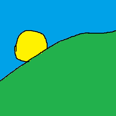
Sun behind a hill (abstract)
For illustrative purposes, I’ve created perhaps the best rendition of a sun peeking over a hill ever. Here, there are three objects in the scene, the sun, the sky, and the hill. For this scene overdraw is potentially present anywhere there is overlap. Consider the region where the hill overlaps the sun. If we had drawn our sun object first, we would have needed to transform, rasterize, shade, and light all the fragments that will later be occluded by the hill. In other words, for every occluded pixel, we potentially pay the entire cost of the pipeline. Of course, we can (and do) mitigate this issue by doing a depth-based sort, rejecting fragments as early as possible when depth-testing, and trying to draw front-to-back. However, remember that for any two objects in a scene, they be overlapping in some parts, but not others. Also, remember that objects are self-occluding.
We have our answer though. Our overdraw is steps 1-5 for all pixels drawn that are ultimately occluded.
Deferred Rendering
An equally ubiquitous technique, deferred rendering cuts the pipeline before step 5. Everything is the same as with forward rendering, but instead of lighting immediately, we save off the results of the per-pixel material evaluation and evaluate lights afterwards, only after the scene’s geometry has been submitted. In practice, the buffers that store all the per-pixel material data is referred to as the gbuffer.
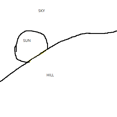
Sun behind a hill (gbuffer rendition)
This gbuffer typically contains material properties like roughness, metalness, albedo, as well as surface data such as orientation. Basically, all the inputs to your BxDF evaluation must be saved off per pixel. Then, the lighting is done afterwards in order to produce the final raster. As before, we play the same game. Where’s the overdraw?
Here, because we evaluate steps 1-4, the overdraw is steps 1-4 for all pixels where geometry was rasterized and the gbuffer was written out. Compared to strict forward rendering, we save the overdraw costs of lighting (step 5).
Z-Prepass
The Z-Prepass is a nearly ubiquitous improvement generally tacked on to either forward or deferred renderers. Here, we run step 1 of the pipeline twice. The first time, we save the depth per pixel in a depth buffer, and the second time, we proceed with either forward or deferred rendering for a given fragment only if the fragment depth matches the depth in the depth buffer. Where’s the overdraw?
In this case, the overdraw is step 1 for every pixel (guaranteed, not just occluded pixels), but we avoid the overdraw of steps 2 through 4/5 compared to the deferred and forward pipelines. It should be clear that in a scene where no occlusion is present, the Z-Prepass is a strict negative, however, a general scene with lots of occluders could benefit a great deal.
Analyzing Tradeoffs
Reducing overdraw is one of the primary motivations for introducing a pipeline cut, either early after vertex processing (Z-Prepass), or prior to lighting (deferred). However, each time we perform a cut, we have to keep in mind the following associated costs:
- Draw call count
- GPU memory storage and bandwidth
- Precision
- Shader specialization
- Hardware underutilization
Draw Call Counts
Each cut in the pipeline results in an additional draw call per-object in the scene. Now, granted, this draw call may be a “no-op” once it hits the GPU, but the CPU doesn’t know if an object is occluded at draw time (barring the use of occlusion queries or CPU occlusion). The CPU needs to both record the draw calls themselves in command buffers, and the driver must turn those command buffers into hardware specific commands at submission time (with any necessary validation and associated costs).
Memory Costs
Every time we cut the pipeline, we incur memory storage costs in order to save off intermediate results, and memory bandwidth costs to write out those results and read them back in again. This is analogous to saving off data and reading it back again later on the CPU. If we defer the work, we miss out on any bandwidth savings of having the data hot in cache, or even present in registers. This is especially true on a GPU, where stalls to main-memory stall not just one core of execution but potentially many.
Note that the memory costs of storing intermediate results are effectively mitigated if you needed to consume that data in a different pass.
Precision
Precision is often not mentioned as often, but is an associated tradeoff with memory. Performing a calculation directly in a shader instead of storing out and reading back in intermediate results often affords the best precision. Doing the calculation inline can use full-width registers, whereas we’ll often use reduced precision buffers to store intermediate results to conserve memory. Of course, we can mitigate precision loss by controlling exposure ranges, quantizing data, and other tricks, but this isn’t entirely free.
Shader Specialization
Pipeline cuts often afford the creation of specialized shaders authored to execute particular portions of the pipeline (e.g. lighting). This is important for a number of reasons, but let’s list the most important ones. Having a higher degree of specialization is usually a good thing because:
- it cuts shader permutations
- smaller shaders tend to use fewer registers and have better occupancy characteristics
- fewer shaders implies fewer pipeline state changes and fewer pipline state objects in general
- smaller shaders are easier to debug and faster to compile
- smaller shaders fit in the GPU’s i-cache more easily
Dedicated Hardware Utilization
One thing to be aware of is that an extremely specialized pass will generally not use the hardware in a “balanced” fashion. A modern GPU has unified shader cores, but still has special hardware for texture filtering, memory fetching, vertex attribute interpolation, and more. In addition, GPUs still have specialized caches on top of the specialized execution units. Passes that utilize a small subset of the hardware are in one sense underutilizing the chip. Trying to maximize utilization isn’t a goal so much as speeding up your frame though, so be wary of architecting strictly to improve this. It’s just a nice thing to have in the back of your mind. If you profile your app, find large bubbles at a point where the pass is dominated by memory bandwidth for example, you can potentially optimize the inefficiency by scheduling other less bandwidth-intensive work at the same time.
Another way in which hardware can be poorly utilized is when quads are dispatched by the hardware rasterizer. Each shaded fragment that needs finite-difference gradients for sampling needs “helper lane” threads to be scheduled. GPU compute units can only accommodate a certain number of thread groups at a time (warps or wavefronts), so thread utilization is another metric to watch out for.
Z-Prepass Revisited
Let’s stop and think through a mental exercise for a moment. What are the costs associated with using a Z-Prepass?
On the GPU, having a Z-Prepass implies processing all geometry twice. Thus, if you have really finely subdivided geometry, or if your geometry processing is really expensive relative to your material and lighting pipeline stages, the Z-Prepass may start to be a deoptimization.
On the CPU, we have to record an additional draw call per-object, effectively doubling our draw call count.
In terms of memory, all vertex memory needs to be traversed twice (note that for this reason, it may not be a bad idea to deinterleave vertex positions from the rest of your vertex attributes).
Note that, another answer to the above question is that we should avoid the Z-Prepass if the hardware is already effectively doing a similar optimization already (tile-based deferred rasterizers as on mobile class and some integrated GPUs). This highlights how overdraw is just one angle to analyze any given technique, and we’ll look at more lenses later in this article.
A common variant of the full Z-Prepass is to perform a partial prepass, where only your best occluders are rendered in the prepass and subsequent geometry is depth tested accordingly. This has reduced potential for mitiating overdraw, but also reduced CPU costs. Furthermore, you can’t immediately use a depth buffer produced in this way to perform SSR/SSAO.
Visibility Buffer
We’re a bit better equipped now to tackle another family of techniques related to the so-called “visibility buffer.” Here, we don’t store out just depth as in the Z-Prepass, but we don’t go as far as storing out shaded material data either. Instead, we write out, per-pixel, the information needed to extract the vertices associated with the pixel. There are a number of ways to do this, but we’ll restrict ourselves to just three approaches:
- The Filtered and Culled Visibility Buffer: Store per-pixel depth, hierarchical depth, triangle address (instance/primitive id), vertex data
- A Deferred Material Rendering System: Store per-pixel triangle address, barycentric coordinates
- Virtual Deferred Texturing: Store per-pixel UV address into a virtual texture cache, tangent frame
The analysis of these techniques is incredibly nuanced and easily a blog post on its own, so we’ll endeavor to do only a coarse analysis. Essentially, what’s proposed is that we don’t cut the pipeline just before lighting as with the gbuffer, but instead between steps 2 and 4 depending on the variant.
The overdraw saved is evidently the costs of shading a material (sampling material properties, evaluating it, storing it) as with the Z-Prepass. However, there are potentially significant memory storage and bandwidth savings compared to storing the full gbuffer. Conceptually, this family of techniques essentially cuts the pipeline between the vertex and pixel shader, so we’re on the hook for handling things like computing finite-difference gradients for texture sampling, interpolating attributes, and computing barycentric coordinates (either via intrinsic/SV_Barycentrics or manually).
While we lose a bunch of work that hardware may have done for us, cutting the pipeline here, however, affords one potential optimization, which is loop restructuring.
Loop Restructuring
Let’s clarify the triangle pipeline in terms of the how all the objects in a scene are drawn collectively as opposed to a single triangle.
    For all objects in the scene
        For all triangles per object
        |   For all shadow-casting light views
        |       Rasterize the shadow view
        |       For all shadow fragments rasterized
        |       |   Populate depth (and optionally moments) in your shadow atlas
        |
        |   Rasterize the primary view
        |   For all primary fragments rasterized
        |       Interpolate attributes and compute gradients
        |       Extract material surface properties
        |       For all light sources
        |       |   Accumulate light accumulation, sampling shadow maps
Note the emphasis on rasterization above. When we push meshes through the standard vertex shader, we can only rasterize a single view at a time. That means each loop iteration with rasterization above corresponds to 1 + N draw calls (minus whatever is saved through instancing).
When performing the rasterization yourself however, you aren’t restricted in this way and can rasterize as many views as you like. This accesses your position data in a more coherent fashion, and reduces CPU load needed to record and dispatch draw calls that scale proportionally with your shadow caster count.
Whether or not this is a “win” over the typical deferred/forward approach will depend on the scene and quality of your implementation. The more views you have (VR also counts) and the more shadow casters you have, the more attractive the visibility buffer will look. Conversely, if you aren’t rasterizing lots of views and have a low quality software rasterizer (without hierarchical culling and a number of other important optimizations), you’re unlikely to beat the hardware rasterizer, especially when you consider what you’re giving up (vertex attribute interpolation, gradients, etc.).
Tiled Lighting
As a final mini-exercise, let’s touch quickly on the “main ideas” behind the tiled lighting algorithm. When performing tiled lighting, we break up the “for all light sources” loop above into two separate loops. In an initial light prepass, we compute light visibility on a per-tile basis. Then in a secondary loop, we accumulate the irradiance per tile fragment, considering only the lights known to be visible in a given tile.
In view of the tradeoffs discussed above, here are the observations we can make:
- We potentially save dispatching work for lights that don’t effect large swaths of pixels due to visibility
- We need to store additional data per tile corresponding to the lights affecting the tile
- We need to query the light list per tile and write it out. We still traverse the list of all lights once.
- No precision lost because we’re writing lossless data (light ids per tile)
- We can potentially specialize shaders better based on the permutations of light types present per-tile
When encountering variants or extensions of this technique, I recommend performing a similar analysis to understand in a broad sense what tradeoffs are made. Extensions and variants to consider are clustered lighting (subdivision not just in x/y but also along z), and employing a bimodal depth split per-tile.
Summary
This post is admittedly pretty disorganized (sorry!). The main takeaway hopefully is the list of things to have in your back of your mind when trying to understand what the goal of a technique is. Below is a small table with the various considerations discussed above, in addition to other miscellaneous considerations:
| Tradeoff | Description |
|---|---|
| Overdraw/Noops | What work is wasted due to occlusion or visibility? |
| Memory storage | What are storage costs needed to save intermediate results? Can I use those intermediate results elsewhere? |
| Memory bandwidth | How much traffic to transient storage is needed? |
| Precision | What precision is sacrificed? |
| Shader Specialization | Between having granular shaders per step vs a single ubershader, what specialization does the technique afford? |
| Hardware usage | What dedicated hardware is used or forgone (registers, LDS, caches, execution units, etc.)? |
| Coherence | Does the technique permit loop structuring that accesses memory more coherently? |
| Complexity | How many optimizations are needed to make the technique tenable? |
All of the tradeoffs above need to be considered for your project and the content that is needed. Once you understand the broad strokes of the algorithms and “alt pipelines,” you should be able to sprinkle the gamut of optimizations available to each technique (scalarization, depth range splitting, use of APIs such as multidraw, dispatch indirect, etc.).