Implementing the FLIP algorithm
All code implemented for this post is provided under MIT-license here.
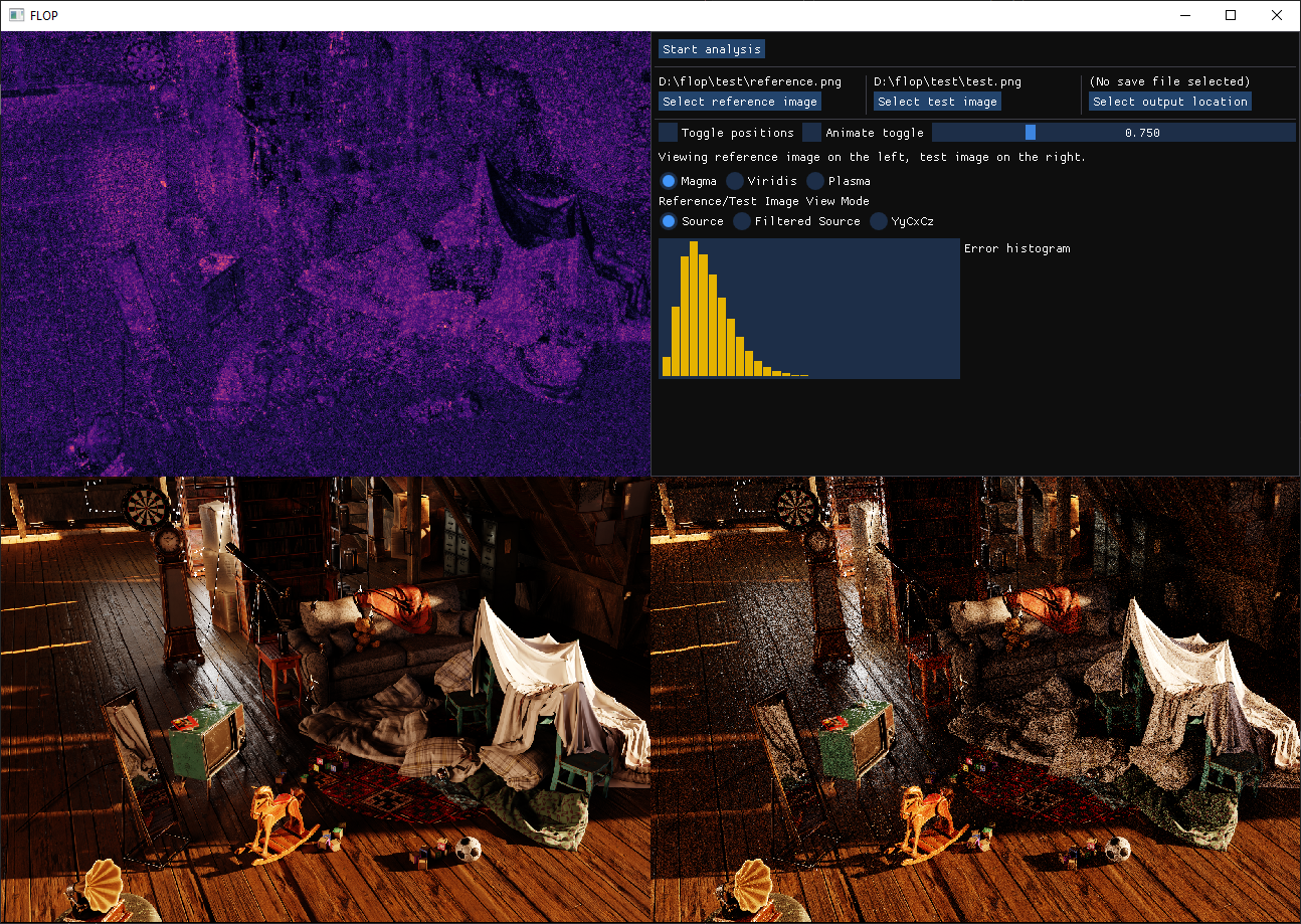
The past couple weekends, I took some time to implement an image delta viewer I am calling “FLOP” as an homage to the paper its implementation is based on (FLIP).
In this short post, I’ll describe the algorithm, and some of the background needed to understand the technique. I’ll also quickly discuss the compute-based implementation, and close off with some thoughts on future direction.
The Problem Statement
Suppose you’re making tweaks to your path tracer, GI system, renderer, whatever. You want to compare before and after shots, and at a glance determine what changed and to what degree. Alternatively, you might have done some optimization work which shouldn’t have changed anything, but you’d like to verify that this is indeed the case.
One approach could be to just use some simple metric to take the difference between RGB values for every pixel on the screen. An example metric might be the Euclidean metric, in which case your delta might look like so:
\[\Delta_E(c, c') = \sqrt{ (c_r - c'_r)^2 + (c_g - c'_b)^2 + (c_b - c'_b)^2}\]Or you might do a Manhattan distance:
\[\Delta_M(c, c') = \left|c_r - c'_r\right| + \left|c_g - c'_g\right| + \left|c_b - c'_b\right|\]Neither choice is wrong per se, but we might ask ourselves if there is a more useful metric we could come up with. Take a look at the screenshot below.
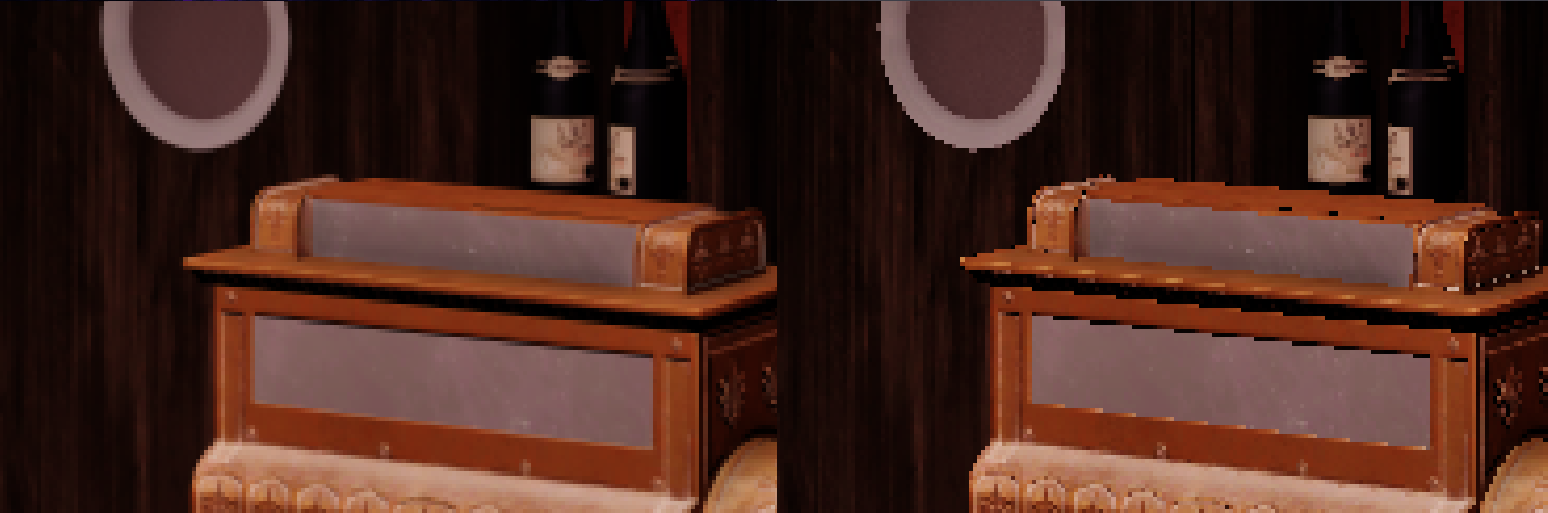
Between the left and the right image, what stands out to you? Chances are, you’re drawn to the poorly anti-aliased edges, some hue-shifts on the bottom portion of the cash register, and speckling in various places. The question to ask is, if I use the metrics defined above (or some other metric I come up), is it the case that two errors computed, say, $0.2$ and $0.4$ necessarily appear twice as different?
Herein lies the issue. Our brains and eyes working together in the Human Vision System (HVS) has its own notions of how to measure differences between color values. Instead of starting from an arbitrary metric, what if we tried to, instead, replicate or approximate the metric the HVS uses instead? This is the problem FLIP aims to solve, and the metric we will describe in this post.
Some facts about color
As a reminder, RGB colors have very little to do with how our eyes actually work, but turn out to be an amazing digital representation of color nonetheless. Contrary to popular belief, we don’t have “spectral cones” in our eyes, which respond to spectral red, spectral green, or spectral blue light respectively. Each of the three cones we possess responds to a range of the visible light spectrum, and these ranges all overlap. As a result, the cones are referred to more often as the L, M, and S cones (referring to long/medium/short wavelengths) as opposed to referencing a specific narrow band of the spectrum by name. The absorbance profiles of the LMS cones effectively convolve with the light incident on our eyes, and combine later with retinal ganglion cells, which ultimately produces a signal our brain perceives as color. The entire pipeline of incident photon to emitted electrical signal is often summarized as the Opponent Process Theory, which while still an approximation, is an amazing model for explaining a host of related color phenomena confirmed experimentally.
Another fact which should be obvious but is worth stating anyways is that cones and rods occupy physical space (they are indeed cells) and so our eyes have a certain resolution when observing a given light field. For example, if you draw two circles on a page and walk sufficiently far away, eventually the dots will appear the same. The monitor or screen you are looking at exploits this fact to give the illusion of smooth lines and surfaces when in actuality, you are looking at a field of discrete illuminants. Furthermore, when observed experimentally, it turns out that our eyes have different resolutions depending on the color and luminance level observed. The experimental data that captures this effect are known as the Contrast Sensitivity Functions (CSF).
Our eyes also perceive differences in color differently depending on brightness levels. (Perceptually) brighter colors appear more “colorful” than darker colors, so differences in chrominance grow with higher intensity. In addition, our eyes are generally keen on picking out large shifts in contrast that manifest as edges or fireflies in our vision.
There are a whole host of other effects that are nicely summarized in this wikipedia page describing what is referred to as the “Color Appearance Model,” some of which are practical to account for in pursuit of our “ideal HVS replicating metric,” and others of which are not. For example, it’d be difficult to account for our eye adaptation process, which adjusts our light sensitivity based on prolonged exposure to a given luminance level.
FLIP
The FLIP metric attempts to account for the following facts:
- Our eyes perceive color according to the opponent process, with red and green sharing one channel (a), blue and yellow sharing another (b), and an achromatic channel which codes for lightness (L).
- Our eyes are more sensitive to chrominance for brighter colors (Hunt effect)
- Our eyes pick out edges and pixel discontinuities
- Our eyes perceive luminance non-linearly
- Our eyes have limited spatial resolution which is hue and lightness dependent
I highly suggest reading the original paper as it is well-written and highly approachable. To summarize the approach though, the pipeline is described roughly as follows:
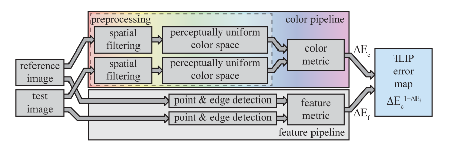
Color difference
First, both images are transfered into YyCxCz space. This space is like CIELAB (also known as L*a*b*), but avoids the non-linear transform meant to mimic the HVS’s response function. We could also call it Lab space as opposed to L*a*b* since the asterisk is used to denote a perceptually mapped coordinate.
Next, in our “linearized CIELAB” space, we filter (aka blur) the images according to kernels derived from the contrast sensitivity functions. The contrast sensitivity functions are defined in the frequency domain, so to make our convolution simpler, we first take them to the spatial domain, and fit them using Gaussians. It turns out that the L and a components are well approximated with a single gaussian, but for b we need the sum of two gaussians. Luckily, deriving these kernel weights can be done offline, and the actual gaussian parameters (amplitude and width) were determined by the NVIDIA researches and provided for us. This filtering explains why Lab is preferred to L*a*b*. Generally when adding values together, you can’t do so if the values themselves don’t combine linearly (same problem as trying to blend sRGB values that have been gamma-transferred).
After filtering, we adjust the chrominance values depending on the lightness coordinate to account for the Hunt effect. Essentially, the transformation amounts to scaling the a and b coordinates by a L with the appropriate normalization. This produces our “Hunt-adjusted” color values (in CIELAB L*a*b* space now instead or the lineared space) that we can compute the difference between. The metric used in this step is the HyAB distance, given below:
\[\Delta_{HyAB}(C, C') = \left|C_L - C'_L\right| + \sqrt{(C_a - C'_a)^2 + (C_b - C'_b)^2}\]In words, take the absolute difference between lightness values and add that to the Euclidean distance between the chrominance values. The rationale for the use of this metric is that it works regardless of the distance between the colors $C$ and $C’$ being compared. Beyond this, some additional normalizing and remapping is done to get the “color distance” value into a nice $[0, 1]$ range.
Feature detection
In parallel to computing the color difference, we can also perform a separate set of convolutions to detect edges and point discontinuities in our image. As with the contrast filters, the feature filters are based on the physiology of the HVS and the kernels can be computed offline (for a fixed pixel density and screen distance). To detect edge features, we convolve with the first derivative of a gaussian, and to detect point features, we convolve with the second derivative of a gaussian.
Fortunately, both of these filters are separable, just as normal gaussian is. I’m embarrassed to say I worked out the math myself before realizing that the original FLIP repository has a helpful pdf describing the derivations. Intuitively though, the way it works is by convolving in one-dimension with the 1D gaussian derivatives, than blurring that with a gaussian when convolving in the vertical direction (and vice versa) before combining the results.
At the end of the day though, after the feature detection portion of the pipeline is done, you end up with two maps: a color difference map, and a feature map. Both maps are filtered in accordance to the actual resolution and sensitivies of a typical eye (again, assuming a particular pixel density and viewing distance, which can be configured).
Putting it all together
The final step is to amplify color differences based on features we detect. This way, we account for both effects and summarize the combination in a nice $[0, 1]$ quantity. The approach take by FLIP is to raise the color difference to one-minus-the-feature-difference. That is, a complete absence of a feature leaves the color difference unperturbed. A saturated feature pushes the combined error to $1$.
Implementation
The first thing I did was play around with a number of the formulae in a simple script to ensure I understood the algorithm and could reproduce the results. The script I used to evaluate things is here which I have in a rough form in an Observable interactive tool. The comments here more or less describe how all the weights were determined from empirically fit parameters provided by the paper.
The actual convolution passes themselves are all implemented as compute shaders. The CSF filter used to smooth out contrast changes our eyes can’t detect is shown below:
// Defines common color space transformation functions
#include "Common.hlsli"

// The CSF Gaussian blurs are done in two passes. First, we blur in the x direction,
// then in the y direction (this choice is arbitrary since the Gaussian decomposition
// is commutes).

// These values are computed using the flip_kernels.js script
static const float sy_kernel[] = {
    0.39172750, 0.24189219, 0.05695543, 0.00511357, 0.00017506
    };
static const float sx_kernel[] = {
    0.36889303, 0.24056897, 0.06672016, 0.00786960, 0.00039475
    };
static const float sz_kernel1[] = {
    0.11730367, 0.11084383, 0.09352148, 0.07045487, 0.04739261, 0.02846493, 0.01526544, 0.00730985, 0.00312541, 0.00119318
};
static const float sz_kernel2[] = {
    0.08301017, 0.07581780, 0.05776847, 0.03671896, 0.01947017, 0.00861249, 0.00317810, 0.00097833, 0.00025124, 0.00005382
};

#define KERNEL_RADIUS 9
#define INNER_RADIUS 4

#ifdef DIRECTION_X
#define DIRECTION 0
#endif

#ifdef DIRECTION_Y
#define DIRECTION 1
#endif

#ifndef DIRECTION
#error "DIRECTION not specified. Specify DIRECTION=0 for a horizontal blur, and DIRECTION=1 for a vertical blur"
#endif

#define THREAD_COUNT 64
#if THREAD_COUNT < 2 * KERNEL_RADIUS
#error "THREAD_COUNT is too small for this implementation to work correctly"
#endif

struct PushConstants
{
    uint2 extent;
    uint input;
    uint output;
};
[[vk::push_constant]]
PushConstants constants;

[[vk::binding(1)]]
RWTexture2D<float4> rwtextures[];

groupshared float4 data[KERNEL_RADIUS * 2 + THREAD_COUNT];

#if DIRECTION == 0
[numthreads(THREAD_COUNT, 1, 1)]
#else
[numthreads(1, THREAD_COUNT, 1)]
#endif
void CSMain(uint3 id : SV_DispatchThreadID, int3 gtid : SV_GroupThreadID, int3 gid : SV_GroupID)
{
    RWTexture2D<float4> input = rwtextures[constants.input];
    RWTexture2D<float4> output = rwtextures[constants.output];

    const uint lds_offset = gtid[DIRECTION] + KERNEL_RADIUS;

    // First, fetch all texture values needed starting with the central values
    int2 uv = clamp(id.xy, int2(0, 0), constants.extent - int2(1, 1));
#ifdef DIRECTION_X
    data[lds_offset] = input[uv].rgbb;
#else
    data[lds_offset] = input[uv].rgba;
#endif

    // Now, fetch the front and back of the window
    if (gtid[DIRECTION] < KERNEL_RADIUS * 2)
    {
        uint offset;
        if (gtid[DIRECTION] < KERNEL_RADIUS)
        {
#if DIRECTION == 0
            uv = int2(gid.x * THREAD_COUNT, id.y);
#else
            uv = int2(id.x, gid.y * THREAD_COUNT);
#endif
            uv[DIRECTION] = uv[DIRECTION] - gtid[DIRECTION] - 1;
            offset = KERNEL_RADIUS - gtid[DIRECTION] - 1;
        }
        else
        {
#if DIRECTION == 0
            uv = int2((gid.x + 1) * THREAD_COUNT, id.y);
#else
            uv = int2(id.x, (gid.y + 1) * THREAD_COUNT);
#endif
            uv[DIRECTION] = uv[DIRECTION] + gtid[DIRECTION] - KERNEL_RADIUS;
            offset = THREAD_COUNT + gtid[DIRECTION];
        }

        uv = clamp(uv, int2(0, 0), constants.extent - int2(1, 1));
#if DIRECTION == 0
        data[offset] = input[uv].rgbb;
#else
        data[offset] = input[uv].rgba;
#endif
    }

    GroupMemoryBarrierWithGroupSync();
    // At this point, all input values in our sliding window are in LDS and ready to use

    float4 color = data[lds_offset] * float4(sx_kernel[0], sy_kernel[0], sz_kernel1[0], sz_kernel2[0]);

    [unroll]
    for (int i = 1; i != INNER_RADIUS; ++i)
    {
        float2 xy = data[lds_offset - i].xy + data[lds_offset + i].xy;
        color.xy += float2(sy_kernel[i], sx_kernel[i]) * xy;
    }

    [unroll]
    for (int j = 1; j != KERNEL_RADIUS; ++j)
    {
        float2 zw = data[lds_offset - j].z + data[lds_offset + j].z;
        color.zw += float2(sz_kernel1[j], sz_kernel2[j]) * zw;
    }

    // Write out the result
    if (id.x < constants.extent.x && id.y < constants.extent.y)
    {
#if DIRECTION == 0
        output[id.xy] = color;
#else
        // Now that we've finished the blur passes, convert out of YyCxCz back to sRGB
        output[id.xy] = float4(linearized_Lab_to_rgb(float3(color.rg, color.z + color.w)), 1.0);
#endif
    }
}
I wouldn’t say this is necessarily the best way to implement a convolution, but is simple enough to get the job done. Effectively, we load for each warp/wavefront all the values in a window centered on the segment of the image assigned to the warp. As we are implementing the convolutions in two passes (via the Convolution theorem), this is a 1-dimensional window. The values we load are stored in groupshared memory (LDS) for reuse by all the threads in the warp. Finally, we perform a weighted sum for each active thread and export the result.
I then implemented a similar kernel for the feature detection, although this convolution is slightly more convoluted (heh) because the first and second derivatives depend on the regular gaussian kernel as well.
In the second pass of the feature filter, I combine the results with the color error map as described above:
// We can now compare features and use differences in edges and points detected to
// amplify the color error

float2 feature_delta = abs(features2 - features1);
// NOTE: this 0.5 value can be configurable to amplify or dampen error due to feature differences
float feature_error = pow(max(feature_delta.x, feature_delta.y) / sqrt(2), 0.5);

float color_error = output[id.xy].r;

// The moment we've all been waiting for
float flip_error = pow(color_error, 1.0 - feature_error);

output[id.xy].rgb = flip_error;
All that’s left is to put it all together with a modest ImGUI interface, and we have the FLOP tool seen at the start of the article.
Conclusion
Aside from all the awesome color theory, I think one takeaway that’s worth mentioning is that paper reproducibility is awesome. It’s not often I can take a paper and implement the whole thing end to end in a couple weekends, and this speaks more to the strength of the original paper itself. The theory and process used to develop this algorithm aren’t simple either, and the results speak for themselves. So, hats of to the NVIDIA research team for sharing this incredible work and making it available to us to learn from.